❌

Normal view

A Visual Guide to Attention Variants in Modern LLMs

22 March 2026 at 11:55

I had originally planned to write about DeepSeek V4. Since it still hasn’t been released, I used the time to work on something that had been on my list for a while, namely, collecting, organizing, and refining the different LLM architectures I have covered over the past few years.

So, over the last two weeks, I turned that effort into an LLM architecture gallery (with 45 entries at the time of this writing), which combines material from earlier articles with several important architectures I had not documented yet. Each entry comes with a visual model card, and I plan to keep the gallery updated regularly.

You can find the gallery here: https://sebastianraschka.com/llm-architecture-gallery/
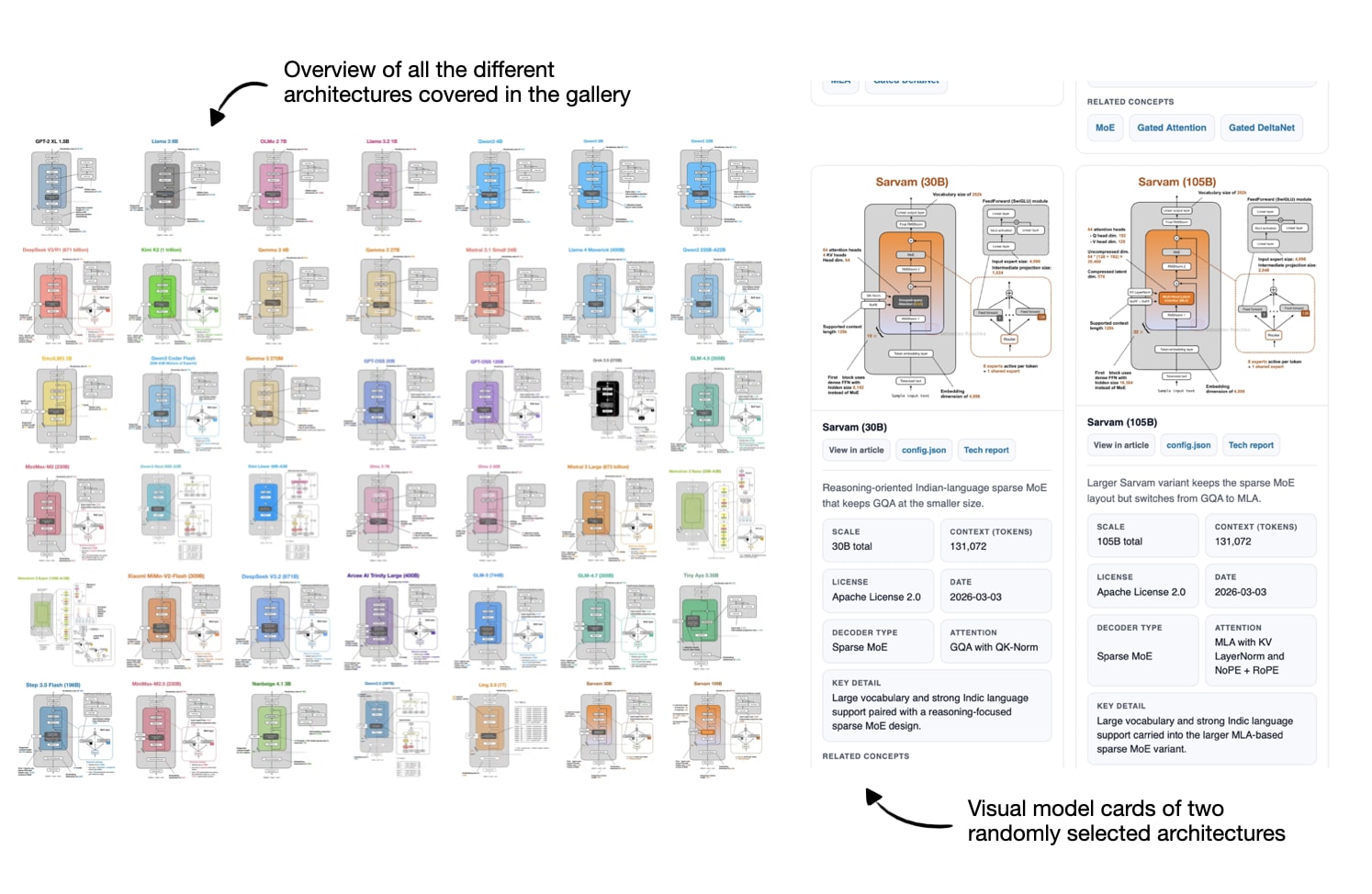
Figure 1: Overview of the LLM architecture gallery and its visual model cards.

After I shared the initial version, a few readers also asked whether there would be a poster version. So, there is now a poster version via Redbubble. I ordered the Medium size (26.9 x 23.4 in) to check how it looks in print, and the result is sharp and clear. That said, some of the smallest text elements are already quite small at that size, so I would not recommend the smaller versions if you intend to have everything readable.
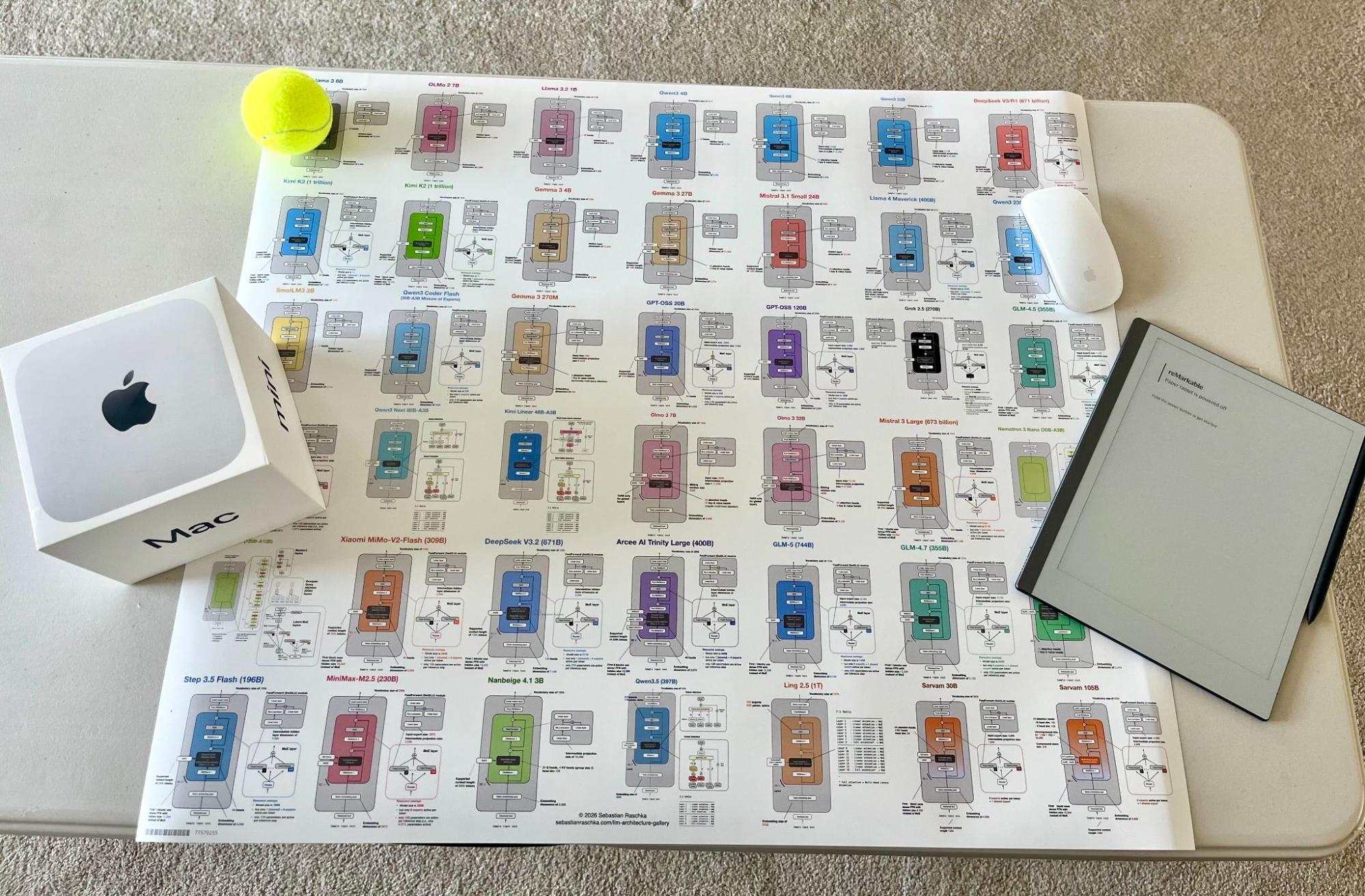
Figure 2: Poster version of the architecture gallery with some random objects for scale.

Alongside the gallery, I was/am also working on short explainers for a few core LLM concepts.

So, in this article, I thought it would be interesting to recap all the recent attention variants that have been developed and used in prominent open-weight architectures in recent years.

My goal is to make the collection useful both as a reference and as a lightweight learning resource. I hope you find it useful and educational!

1. Multi-Head Attention (MHA)

Self-attention lets each token look at the other visible tokens in the sequence, assign them weights, and use those weights to build a new context-aware representation of the input.

Multi-head attention (MHA) is the standard transformer version of that idea. It runs several self-attention heads in parallel with different learned projections, then combines their outputs into one richer representation.
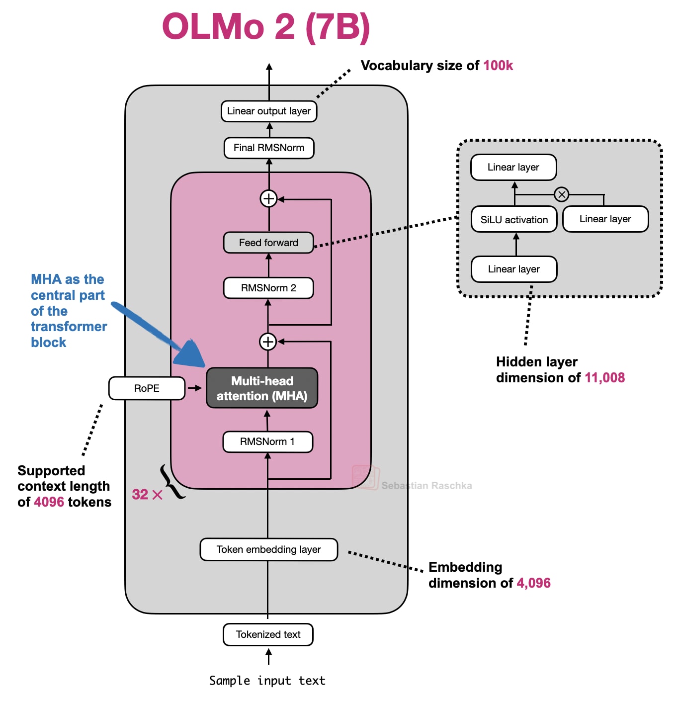
Figure 3: Olmo 2 as an example architecture using MHA.

The sections below start with a whirlwind tour of explaining self-attention to explain MHA. It’s more meant as a quick overview to set the stage for related attention concepts like grouped-query attention, sliding window attention, and so on. If you are interested in a longer, more detailed self-attention coverage, you might like my longer Understanding and Coding Self-Attention, Multi-Head Attention, Causal-Attention, and Cross-Attention in LLMs article.

EXAMPLE ARCHITECTURES

GPT-2, OLMo 2 7B, and OLMo 3 7B

1.2 Historical Tidbits And Why Attention Was Invented

Attention predates transformers and MHA. Its immediate background is encoder-decoder RNNs for translation.

In those older systems, an encoder RNN would read the source sentence token by token and compress it into a sequence of hidden states, or in the simplest version into one final state. Then the decoder RNN had to generate the target sentence from that limited summary. This worked for short and simple cases, but it created an obvious bottleneck once the relevant information for the next output word lived somewhere else in the input sentence.

In short, the limitation is that the hidden state can’t store infinitely much information or context, and sometimes it would be useful to just refer back to the full input sequence.

The translation example below shows one of the limitations of this idea. For instance, a sentence can preserve many locally reasonable word choices and still fail as a translation when the model treats the problem too much like a word-by-word mapping. (The top panel shows an exaggerated example where we translate the sentence word by word; obviously, the grammar in the resulting sentence is wrong.) In reality, the correct next word depends on sentence-level structure and on which earlier source words matter at that step. Of course, this could still be translated fine with an RNN, but it would struggle with longer sequences or knowledge retrieval tasks because the hidden state can only store so much information as mentioned earlier.
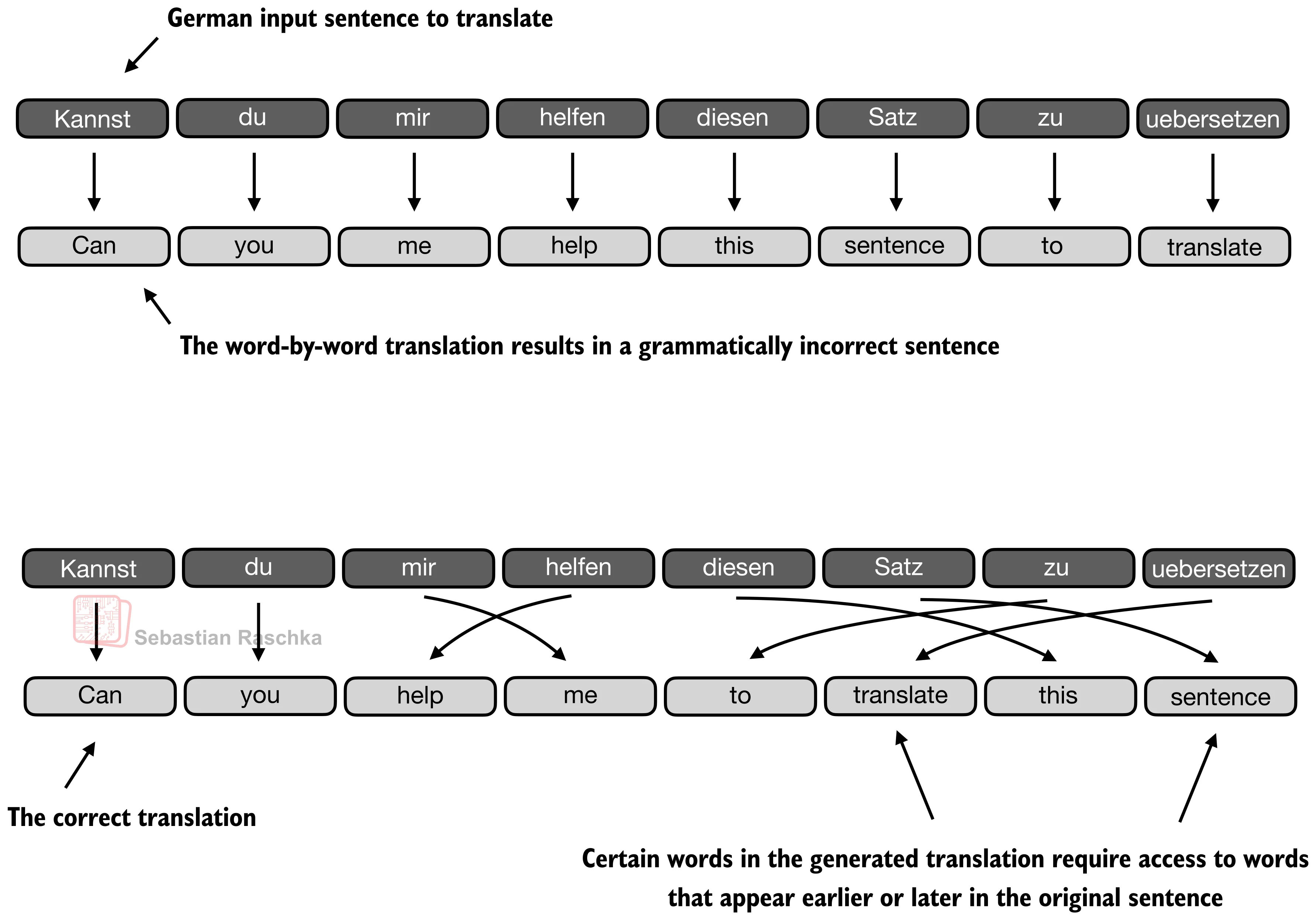
Figure 4: Translation can fail even when many individual word choices look reasonable because sentence-level structure still matters (Original source LLMs-from-scratch).

The next figure shows that change more directly. When the decoder is producing an output token, it should not be limited to one compressed memory path. It should be able to reach back to the more relevant input tokens directly.
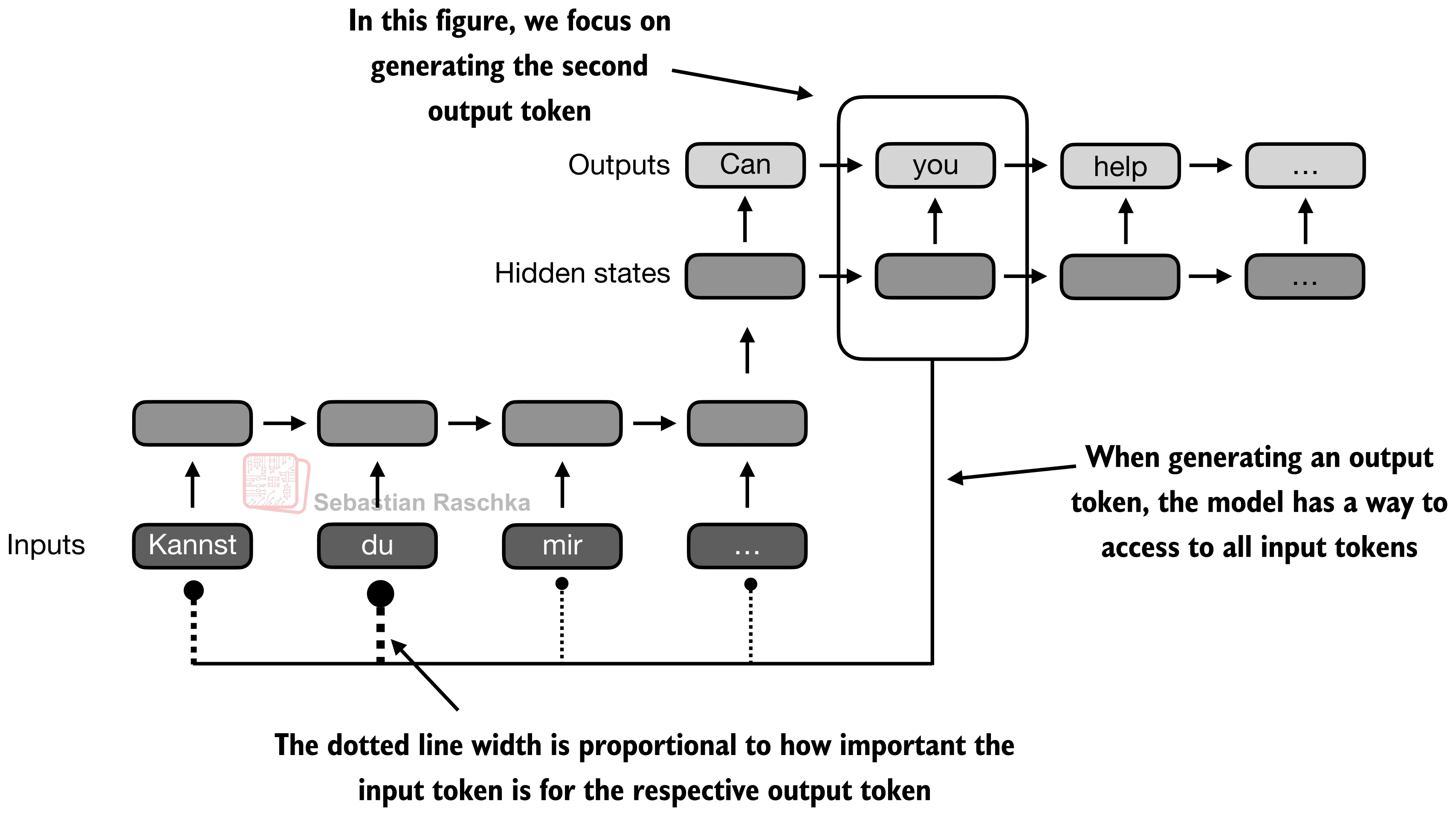
Figure 5: Attention breaks the RNN bottleneck by letting the current output position revisit the full input sequence instead of relying on one compressed state alone (Original source LLMs-from-scratch).

Transformers keep that core idea from the aforementioned attention-modified RNN but remove the recurrence. In the classic Attention Is All You Need paper, attention becomes the main sequence-processing mechanism itself (instead of being just part of an RNN encoder-decoder.)

In transformers, that mechanism is called self-attention, where each token in the sequence computes weights over all other tokens and uses them to mix information from those tokens into a new representation. Multi-head attention is the same mechanism run several times in parallel.

1.3 The Masked Attention Matrix

For a sequence of T tokens, attention needs one row of weights per token, so overall we get a T x T matrix.

Each row answers a simple question. When updating this token, how much should each visible token matter? In a decoder-only LLM, future positions are masked out, which is why the upper-right part of the matrix is grayed out in the figure below.

Self-attention is fundamentally about learning these token-to-token weight patterns, under a causal mask, and then using them to build context-aware token representations.
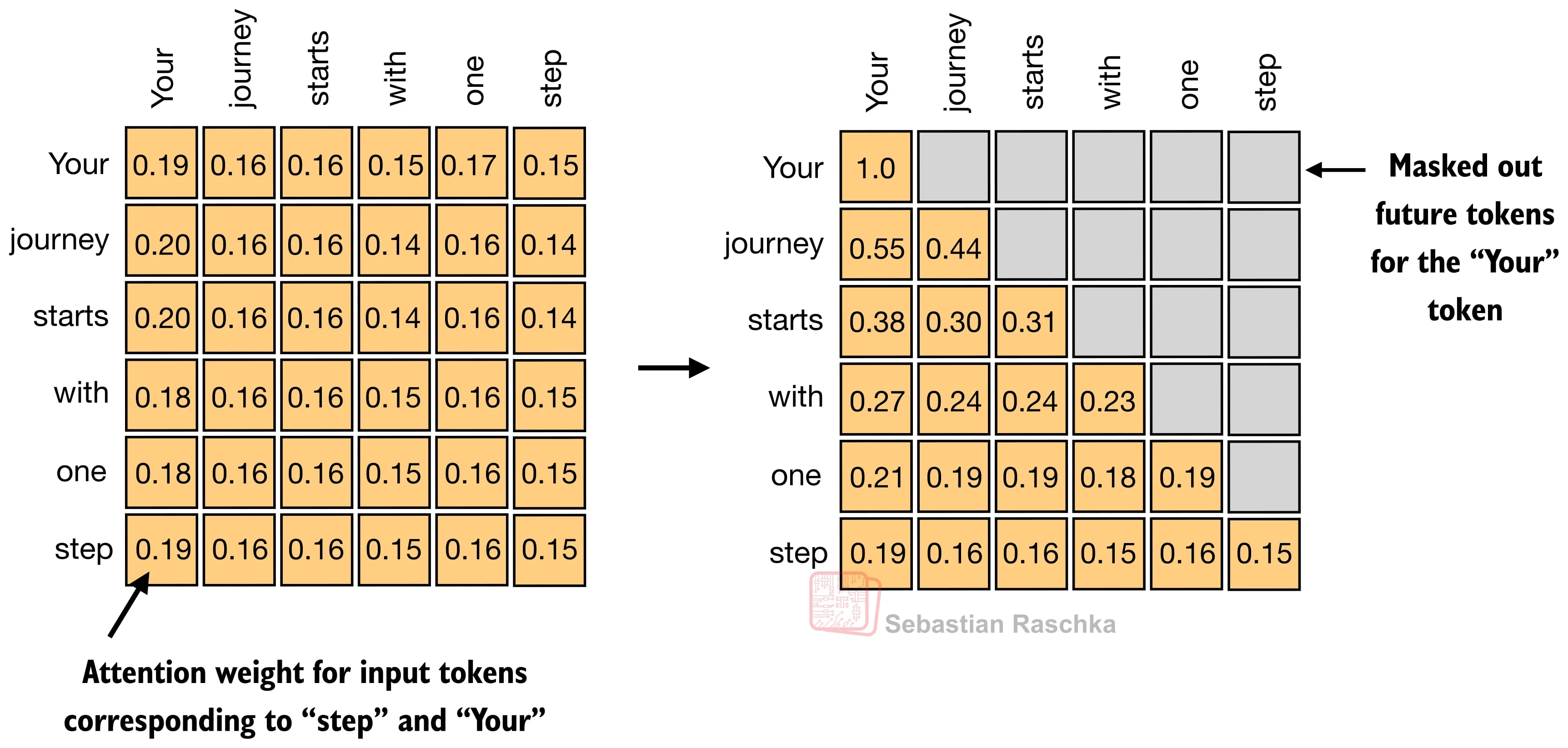
Figure 6: A concrete masked attention matrix where each row belongs to one token, each entry is an attention weight, and future-token entries are removed by the causal mask (Original source Understanding and Coding Self-Attention).

1.4 Self-Attention Internals

The next figure shows how the transformer computes the attention matrix (A) from the input embeddings X, which is then used to produce the transformed inputs (Z).

Here Q, K, and V stand for queries, keys, and values. The query for a token represents what that token is looking for, the key represents what each token makes available for matching, and the value represents the information that gets mixed into the output once the attention weights have been computed.

The steps are as follows:

  • Wq, Wk, and Wv are weight matrices that project the input embeddings into Q, K, and V

  • QK^T produces the raw token-to-token relevance scores

  • softmax converts those scores into the normalized attention matrix A that we discussed in the previous section

  • A is applied to V to produce the output matrix Z

Note that the attention matrix is not a separate hand-written object. It emerges from Q, K, and softmax.
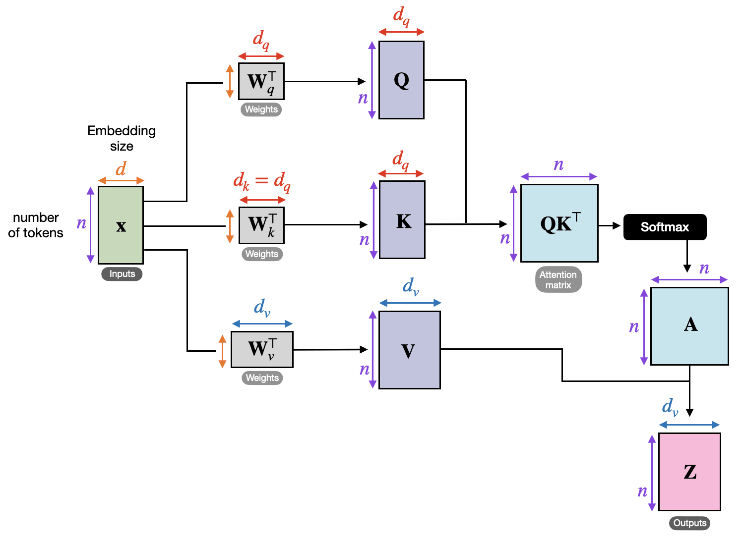
Figure 7: The full single-head pipeline, from input embeddings X to the normalized attention matrix A and output representations Z (Original source Understanding and Coding Self-Attention).

The next figure shows the same concept as the previous figure but the attention matrix computation is hidden inside the “scaled-dot-product attention” box, and we perform the computation only for one input token instead of all input tokens. This is to show a compact form of self-attention with a single head before extending this to multi-head attention in the next section.
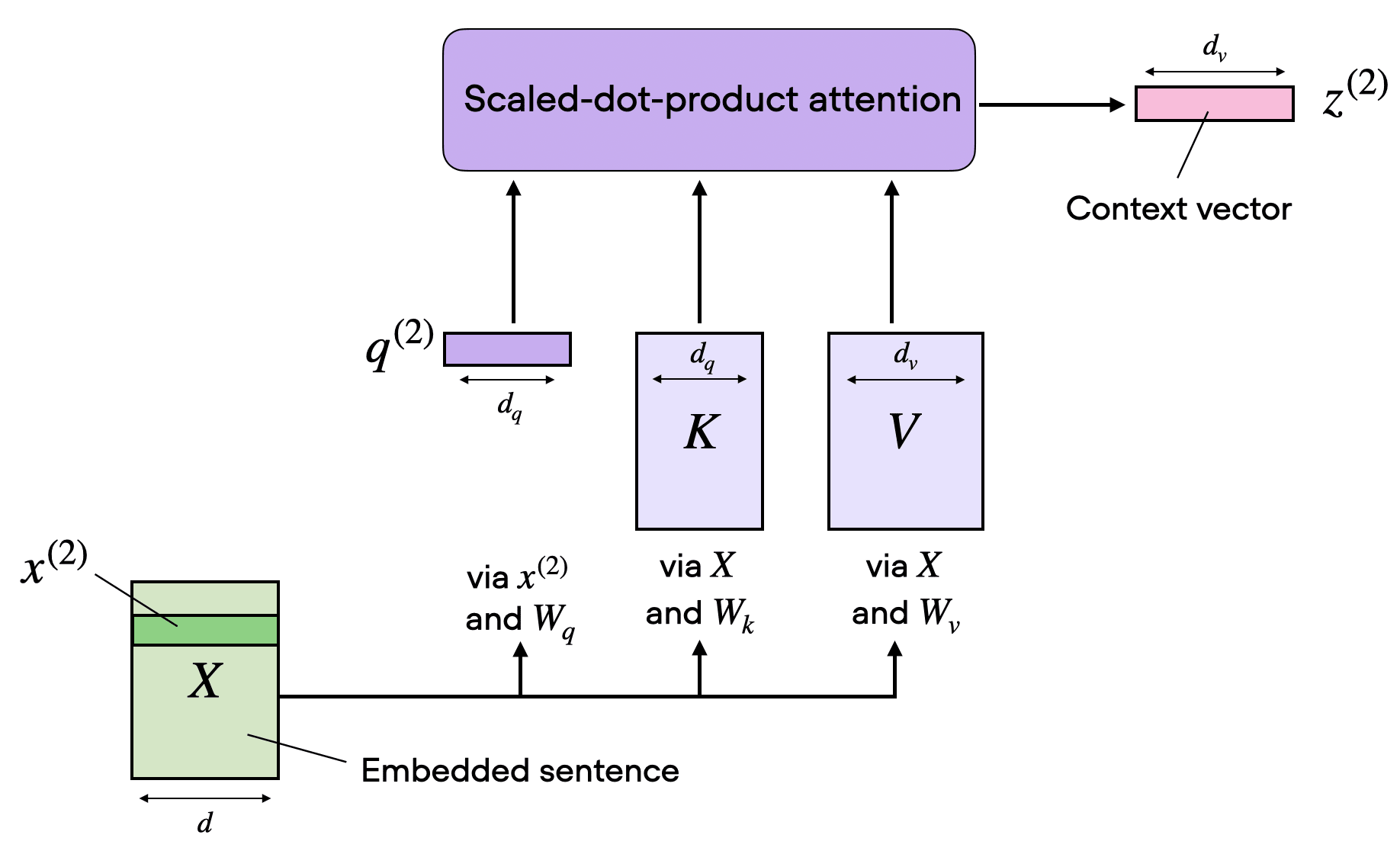
Figure 8: One attention head is already a complete mechanism. One set of learned projections produces one attention matrix and one context-aware output stream (Original source Understanding and Coding Self-Attention).

1.5 From One Head To Multi-Head Attention

One set of Wq/Wk/Wv matrices gives us one attention head, which means one attention matrix and one output matrix Z. (This concept was illustrated in the previous section.)

Multi-head attention simply runs several of these heads in parallel with different learned projection matrices.

This is useful because different heads can specialize in different token relationships. One head might focus on short local dependencies, another on broader semantic links, and another on positional or syntactic structure.
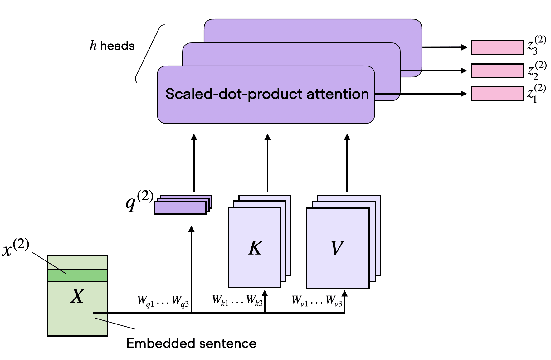
Figure 9: Multi-head attention keeps the same basic attention recipe, but repeats it across several heads in parallel so the model can learn several token-to-token patterns at once (Original source Understanding and Coding Self-Attention).

2. Grouped-Query Attention (GQA)

Grouped-query attention is an attention variant derived from standard MHA. It was introduced in the 2023 paper GQA: Training Generalized Multi-Query Transformer Models from Multi-Head Checkpoints by Joshua Ainslie and colleagues.

Instead of giving every query head its own keys and values, it lets several query heads share the same key-value projections, which makes KV caching much cheaper (primarily as a memory reduction) without changing the overall decoder recipe very much.
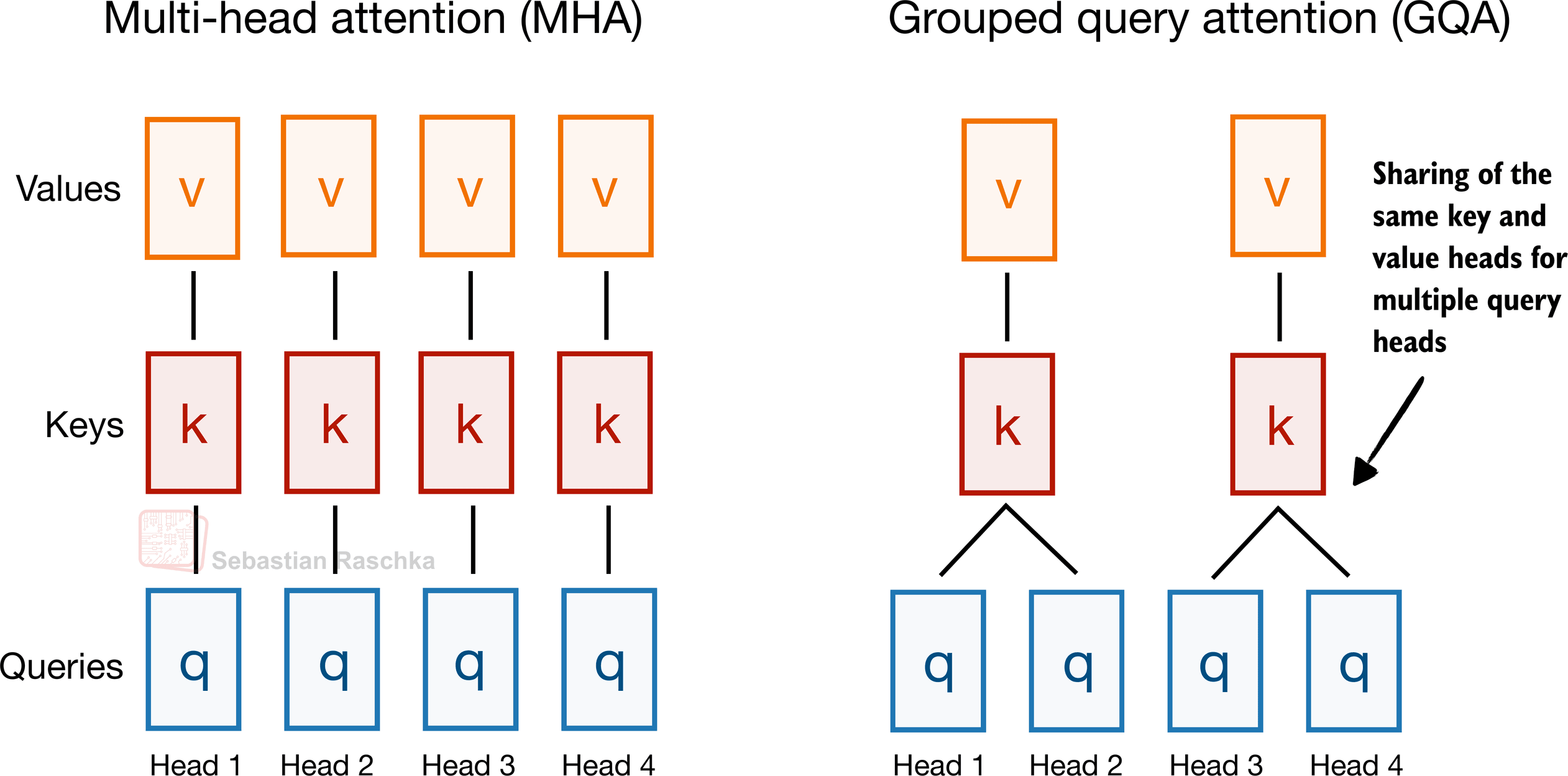
Figure 10: GQA keeps the same overall attention pattern as MHA, but collapses the number of key-value heads by sharing them across multiple query heads (Original source: The Big LLM Architecture Comparison).

EXAMPLE ARCHITECTURES

Dense: Llama 3 8B, Qwen3 4B, Gemma 3 27B, Mistral Small 3.1 24B, SmolLM3 3B, and Tiny Aya 3.35B.
Sparse (Mixture-of-Experts): Llama 4 Maverick, Qwen3 235B-A22B, Step 3.5 Flash 196B, and Sarvam 30B.

2.1 Why GQA Became Popular

In my architecture comparison article, I framed GQA as the new standard replacement for classic multi-head attention (MHA). The reason is that standard MHA gives every head its own keys and values, which is more optimal from a modeling perspective but expensive once we have to keep all of that state in the KV cache during inference.

In GQA, we keep a larger set of query heads, but we reduce the number of key-value heads and let multiple queries share them. That lowers both parameter count and KV-cache traffic without making drastic implementation changes like multi-head latent attention (MLA), which will be discussed later.

In practice, that made and keeps it a very popular choice for labs that wanted something cheaper than MHA but simpler to implement than newer compression-heavy alternatives like MLA.

2.2 GQA Memory Savings

GQA results in big savings in KV storage, since the fewer key-value heads we keep per layer, the less cached state we need per token. That is why GQA becomes more useful as sequence length grows.

GQA is also a spectrum. If we reduce all the way down to one shared K/V group, we are effectively in multi-query attention territory, which is even cheaper but can hurt modeling quality more noticeably. The sweet spot is usually somewhere in between multi-query attention (1 shared group) and MHA (where K/V groups are equal to the number of queries), where the cache savings are large but the modeling degradation relative to MHA stays modest.
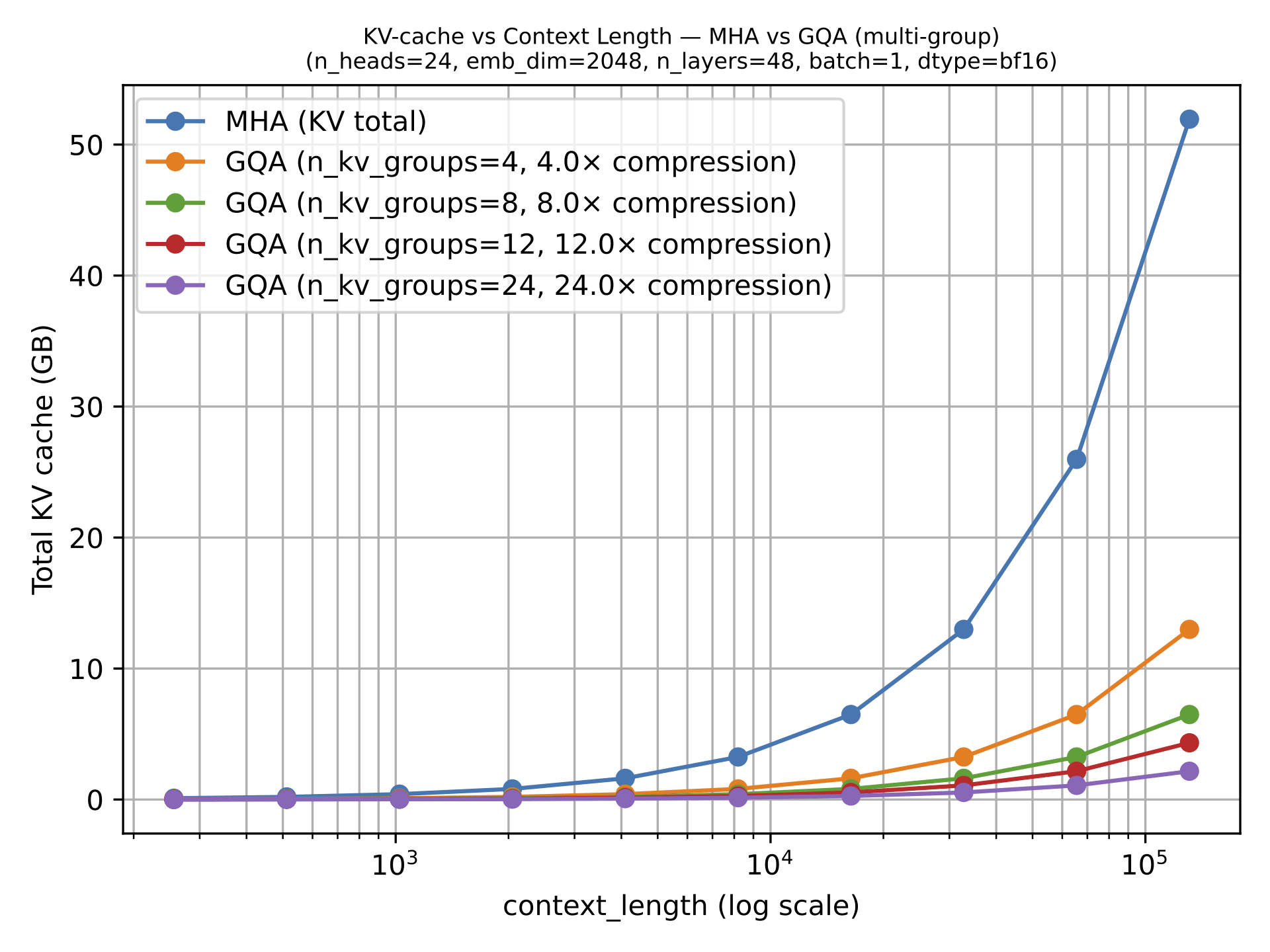
Figure 11: Lower is better. Once the context window grows, KV-cache savings become more pronounced. (Original source: LLMs-from-scratch GQA materials)

2.3 Why GQA Still Matters In 2026

More advanced variants such as MLA are becoming popular because they can offer better modeling performance at the same KV efficiency levels (e.g., as discussed in the ablation studies of the DeepSeek-V2 paper), but they also involve a more complicated implementation and a more complicated attention stack.

GQA remains appealing because it is robust, easier to implement, and also easier to train (since there are fewer hyperparameter tunings necessary, based on my experience).

That is why some of the newer releases still stay deliberately classic here. E.g., in my Spring Architectures article, I mentioned that MiniMax M2.5 and Nanbeige 4.1 as models that remained very classic, using only grouped-query attention without piling on other efficiency tricks. Sarvam is a particularly useful comparison point as well: the 30B model keeps classic GQA, while the 105B version switches to MLA.
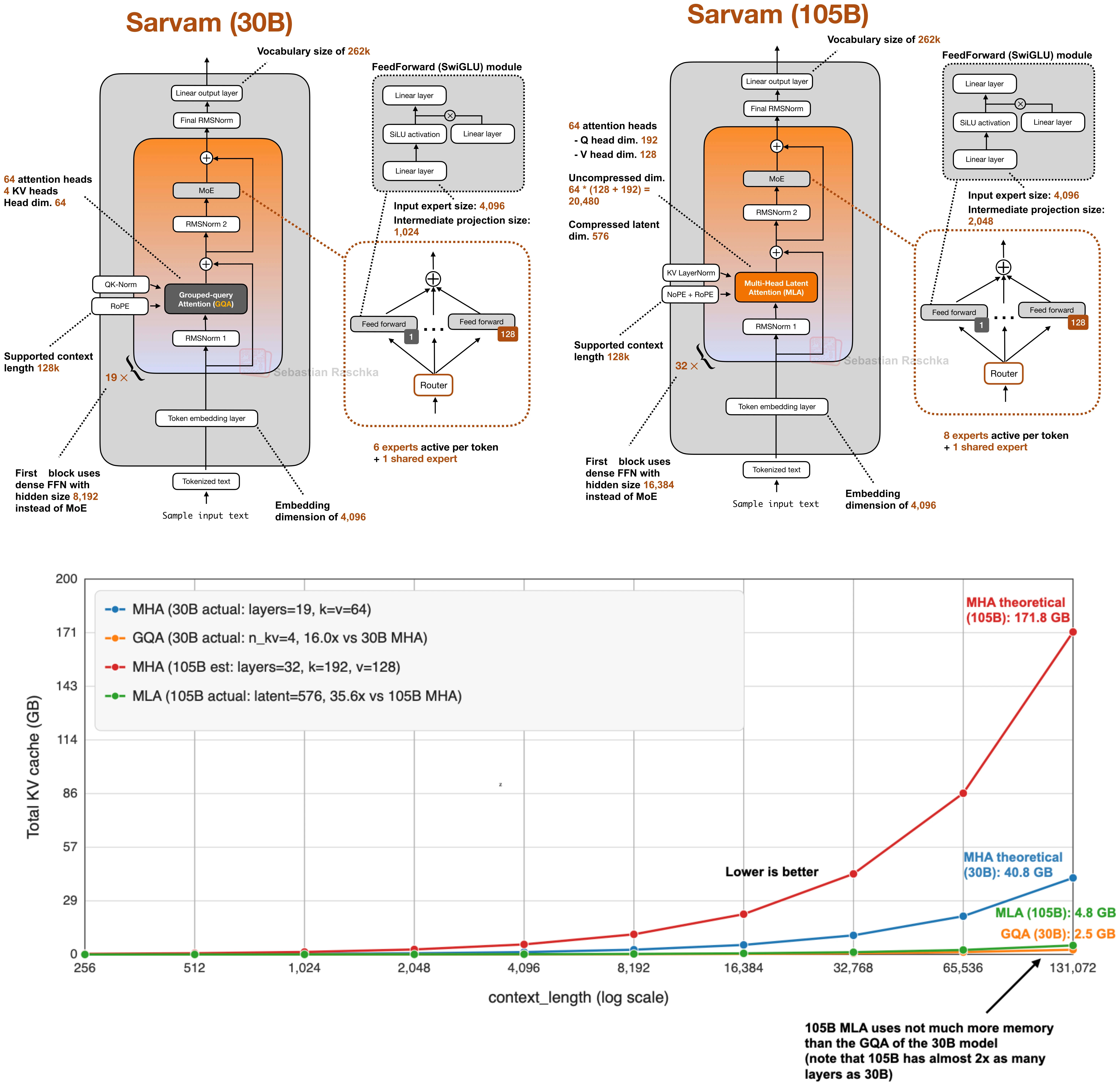
Figure 12: Total KV cache sizes for 105B Sarvam (using MLA) versus 30B Sarvam (using GQA), versus using plain MHA.

3. Multi-Head Latent Attention (MLA)

The motivation behind Multi-head Latent Attention (MLA) is similar to Grouped-Query Attention (GQA). Both are solutions for reducing KV-cache memory requirements. The difference between GQA and MLA is that MLA shrinks the cache by compressing what gets stored rather than by reducing how many K/Vs are stored by sharing heads.
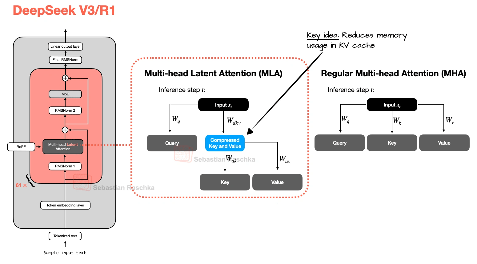
Figure 13: Unlike GQA, MLA does not reduce KV cost by grouping heads. It reduces it by caching a compressed latent representation. Note that it is also applied to the query, which is not shown for simplicity (Original source:The Big LLM Architecture Comparison).

MLA, originally proposed in the DeepSeek-V2 paper, became such a defining DeepSeek-era idea (especially after DeepSeek-V3 and R1). It is more complicated to implement than GQA, more complicated to serve, but nowadays also often more compelling once model size and context length get large enough that cache traffic starts to dominate, because at the same rate of memory reduction, it could maintain better modeling performance (more on that later).

EXAMPLE ARCHITECTURES

DeepSeek V3, Kimi K2, GLM-5, Ling 2.5, Mistral Large 3, and Sarvam 105B

3.1 Compression, Not Sharing

Instead of caching full-resolution key and value tensors as in MHA and GQA, MLA stores a latent representation and reconstructs the usable state when needed. Essentially, it is a cache compression strategy embedded inside attention, as illustrated in the previous figure.

The figure below shows the savings compared to regular MHA.
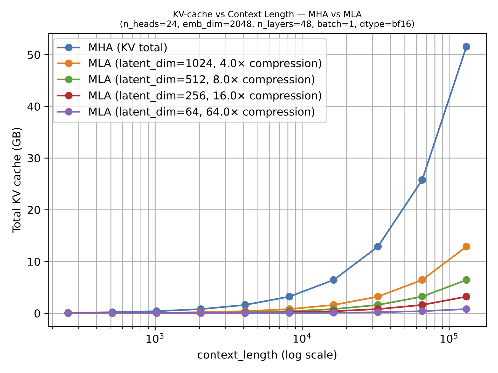
Figure 14: Once context length grows, the savings from caching a latent representation instead of full K/V tensors become very visible (Original source: LLMs-from-scratch MLA section).

3.2 MLA Ablation Studies

The DeepSeek-V2 paper provided some ablations where GQA looked worse than MHA in terms of modeling performance, while MLA held up much better and could even outperform MHA when tuned carefully. That is a much stronger justification than “it (also) saves memory.”

In other words, MLA is a preferable attention mechanism for DeepSeek not just because it was efficient, but because it looked like a quality-preserving efficiency move at large scale. (But colleagues also told me that MLA only works well at a certain size. For smaller models, let’s say <100B, GQA seems to work better, or, is at least easier to tune and get right.)
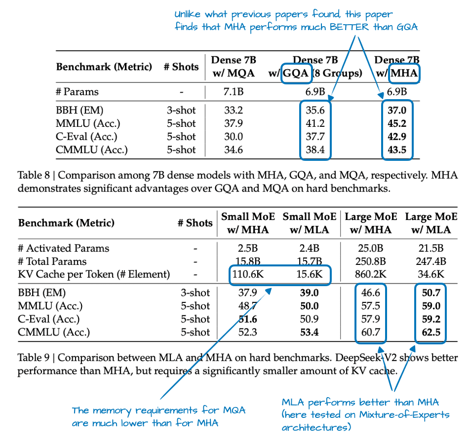
Figure 15: GQA drops below MHA here, while MLA remains competitive and can even slightly outperform it. Underlying paper: DeepSeek-V2.

Below is again the comparison between GQA in 30B Sarvam versus MLA in 105B Sarvam.
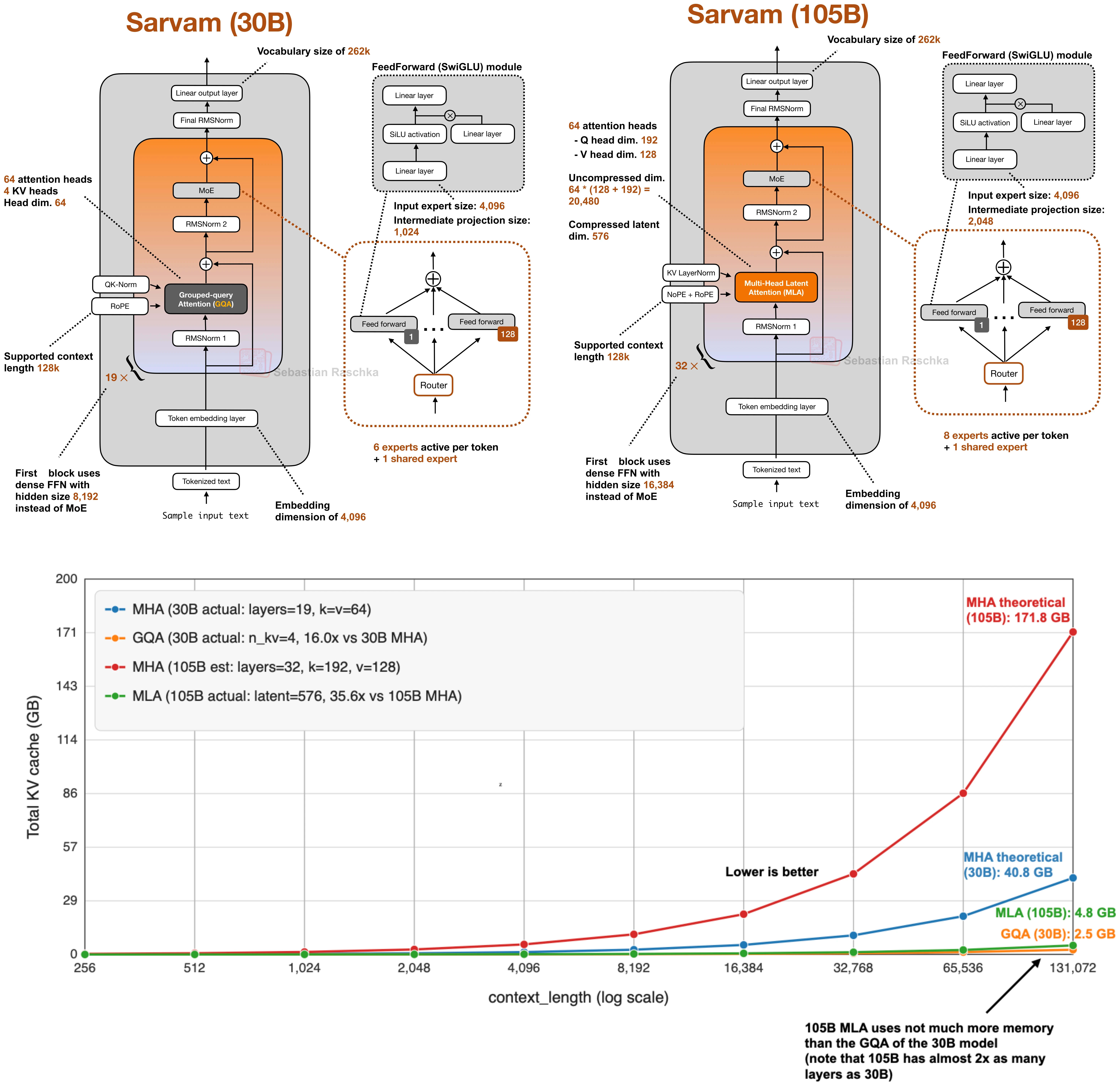
Figure 16: GQA and MLA are solving the same bottleneck from different directions. The tradeoff is simplicity versus better modeling performance for larger models.

3.3 How MLA Spread After DeepSeek

Once DeepSeek V3/R1, V3.1 etc. normalized the design after its introduction in V2, it started showing up in a second wave of architectures. Kimi K2 kept the DeepSeek recipe and scaled it up. GLM-5 adopted MLA together with DeepSeek Sparse Attention (from DeepSeek V3.2). Ling 2.5 paired MLA with a linear-attention hybrid. Sarvam released two models where the 30B model stayed with classic GQA and the 105B model switched to MLA.

That last pair is particularly useful as it puts the technical-complexity discussion aside. I.e., the Sarvam team implemented both variants and deliberately chose to then use GQA for one variant and MLA for the other. So, in a sense, that makes MLA feel less like a theoretical alternative and more like a concrete architectural upgrade path once a family scales up.

4. Sliding Window Attention (SWA)

Sliding window attention reduces the memory and compute cost of long-context inference by limiting how many previous tokens each position can attend to. Instead of attending to the entire prefix, each token only attends to a fixed window of recent tokens around its position. Because attention is restricted to a local token neighborhood, this mechanism is often referred to as local attention.

Some architectures combine these local layers with occasional global attention layers so that information can still propagate across the entire sequence.
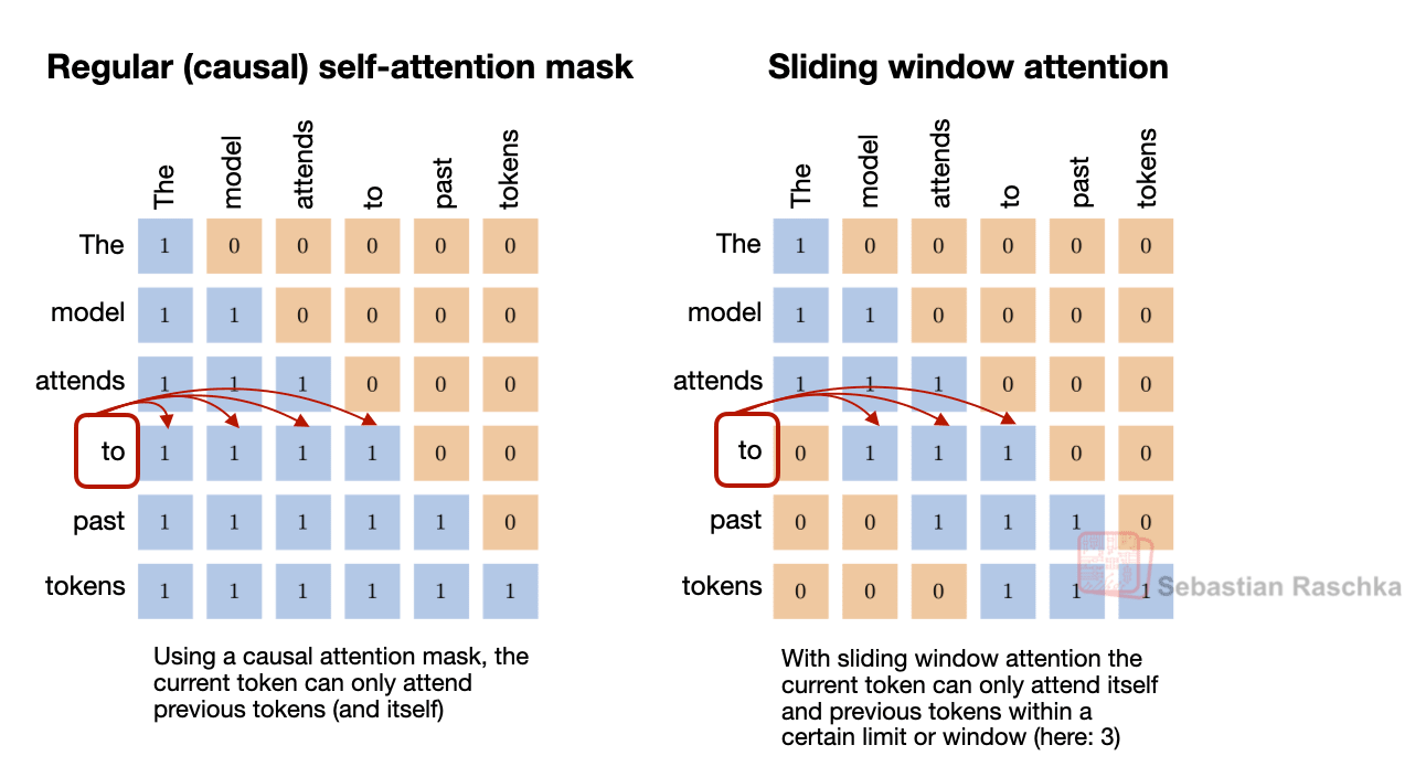
Figure 17: The conceptual shift is simple. Regular attention is global attention, while sliding-window attention is local attention. Global attention lets every token see the full prefix; SWA turns many of those layers into local attention layers (Original source: The Big LLM Architecture Comparison).

EXAMPLE ARCHITECTURES

Gemma 3 27B, OLMo 3 32B, Xiaomi MiMo-V2-Flash, Arcee Trinity, Step 3.5 Flash, and Tiny Aya

4.1 Gemma 3 As A Reference Point

Gemma 3 is still one of the clearest recent SWA examples because it is easy to compare against Gemma 2. Gemma 2 already used a hybrid attention setup with a 1:1 ratio between local and global layers and a 4096-token window. Gemma 3 pushed this further to a 5:1 ratio and reduced the window size to 1024.

The key finding was not that local attention is cheaper, because that was already known. Here, the more interesting takeaway from the Gemma 3 ablation study was that using this more aggressively seemed to hurt modeling performance only slightly.
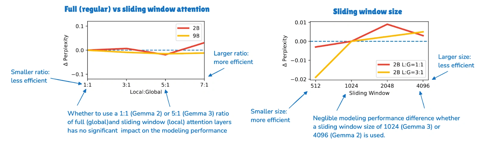
The Gemma ablation study suggests that the smaller window and more aggressive local:global ratio have little effect on perplexity. Underlying paper: Gemma 3 article (Original source: The Big LLM Architecture Comparison).

4.2 The Ratio And Window Size

In practice, saying that a model “uses SWA” does not mean it relies on SWA alone. What usually matters are the local-to-global layer pattern and the attention window size. For example:

  • Gemma 3 and Xiaomi use a 5:1 local-to-global pattern.

  • OLMo 3 and Arcee Trinity use a 3:1 pattern.

  • Xiaomi also uses a window size of 128, which is much smaller, and therefore more aggressive, than Gemma’s 1024.

SWA is essentially a knob that can be tuned more or less aggressively.
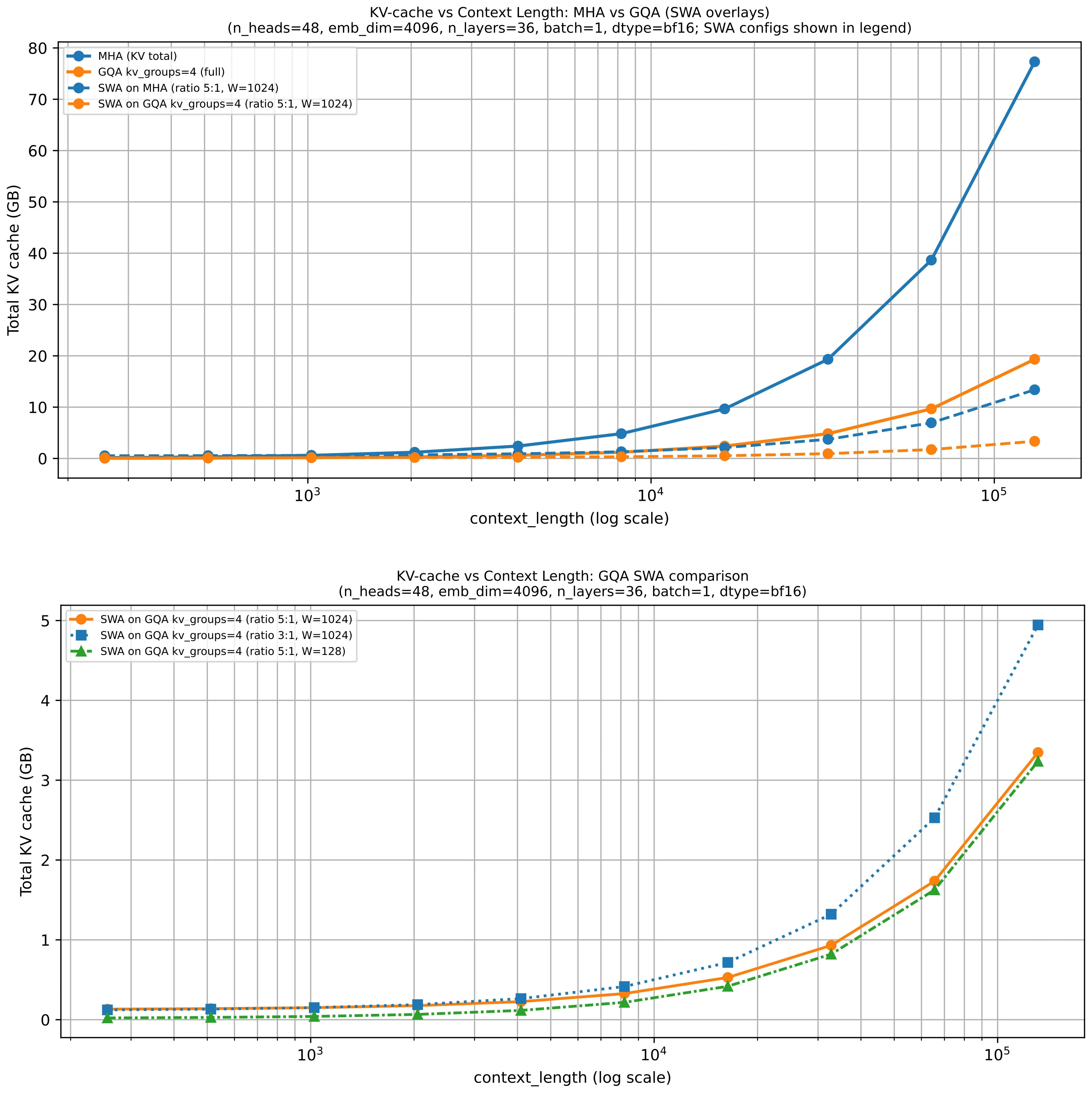
Figure 18: The long-context savings come from turning many full-attention layers into local ones, which reduces how much cached context those layers need to consider (Original source: LLMs-from-scratch SWA materials).

4.3 Combining SWA with GQA

SWA often appears together with GQA because the two ideas address different parts of the same inference problem. SWA reduces how much context a local layer has to consider. GQA reduces how much key-value state each token contributes to the cache.

That is why many recent dense models use both rather than treating them as alternatives. Gemma 3 is again a good reference point here, since it combines sliding window attention with grouped-query attention in the same architecture.

5. DeepSeek Sparse Attention (DSA)

DeepSeek Sparse Attention is one of the architectural changes that appeared in the DeepSeek V3.2 line and later showed up again in GLM-5.

Specifically, DeepSeek V3.2 combines it with Multi-head Latent Attention (MLA), and GLM-5 adopts the same pair for the same general reason, namely, reducing inference cost when context lengths get large.

EXAMPLE ARCHITECTURES

DeepSeek V3.2 and GLM-5

5.1 Changes Relative To Sliding-Window Attention

In sliding-window attention, the current token does not attend to the full prefix but only to a fixed local window. This is the same broad idea behind DeepSeek Sparse Attention, where each token also only attends to a subset of previous tokens.

However, the selected tokens are not determined by a fixed-width local window. Instead, DeepSeek Sparse Attention uses a learned sparse pattern. In short, it uses an indexer-plus-selector setup, where a lightning indexer computes relevance scores, and a token selector keeps only a smaller set of high-scoring past positions.

The way the subset of tokens is selected is the main difference from sliding-window attention. Sliding-window attention hard-codes locality. DeepSeek Sparse Attention still limits attention to a subset, but it lets the model decide which prior tokens are worth revisiting.
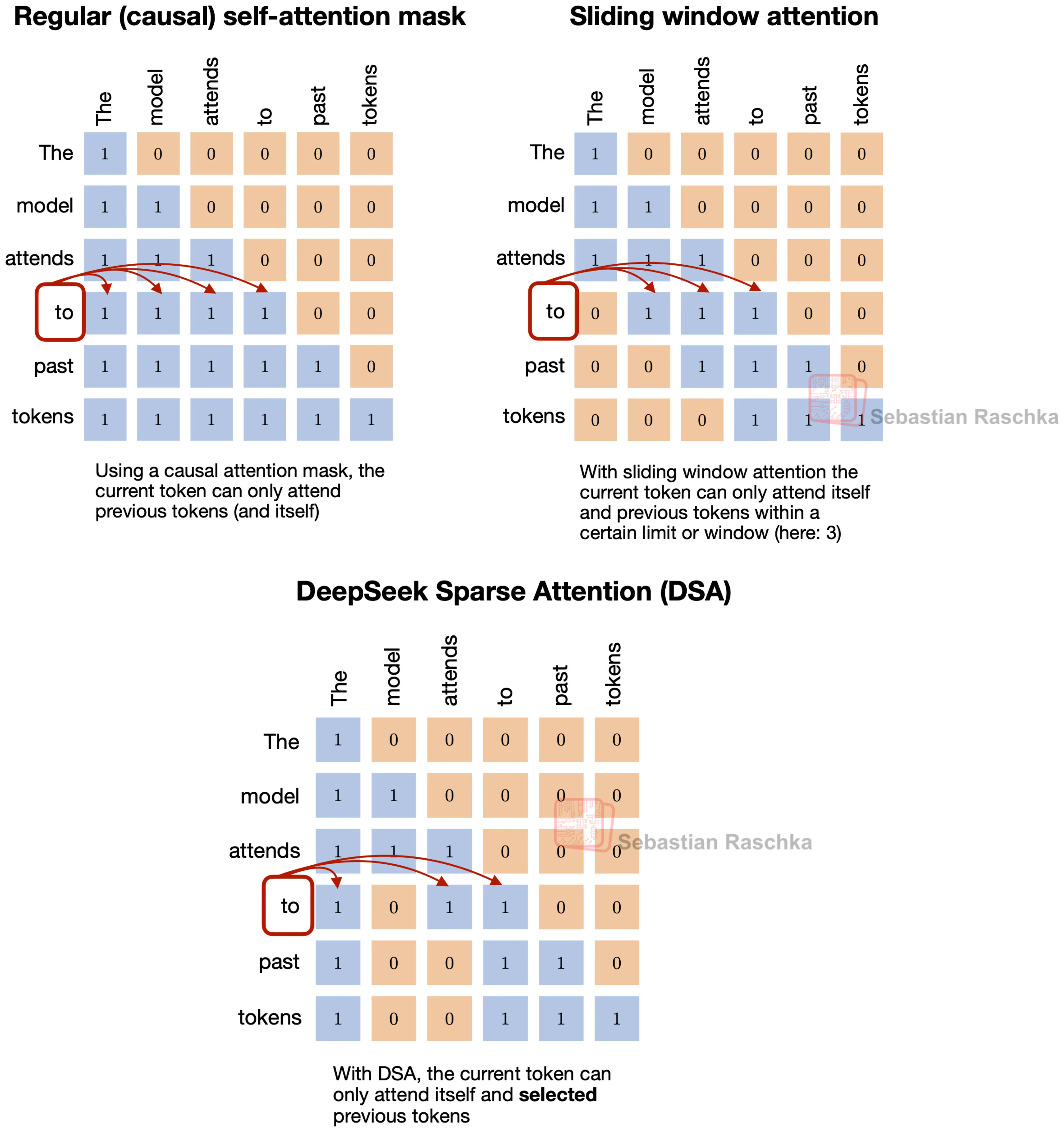
Figure 19: Similar to sliding-window attention, DeepSeek Sparse Attention also restricts each token to a subset of prior tokens, but does not do so with a fixed local window (Original source: From DeepSeek V3 to V3.2: Architecture, Sparse Attention, and RL Updates).

5.2 DeepSeek Sparse Attention and MLA

DeepSeek V3.2 uses both Multi-head Latent Attention (MLA) and DeepSeek Sparse Attention. MLA reduces KV-cache cost by compressing what gets stored. DeepSeek Sparse Attention reduces how much of the prior context the model has to revisit. Put differently, one optimizes the cache representation, the other optimizes the attention pattern on top of it.
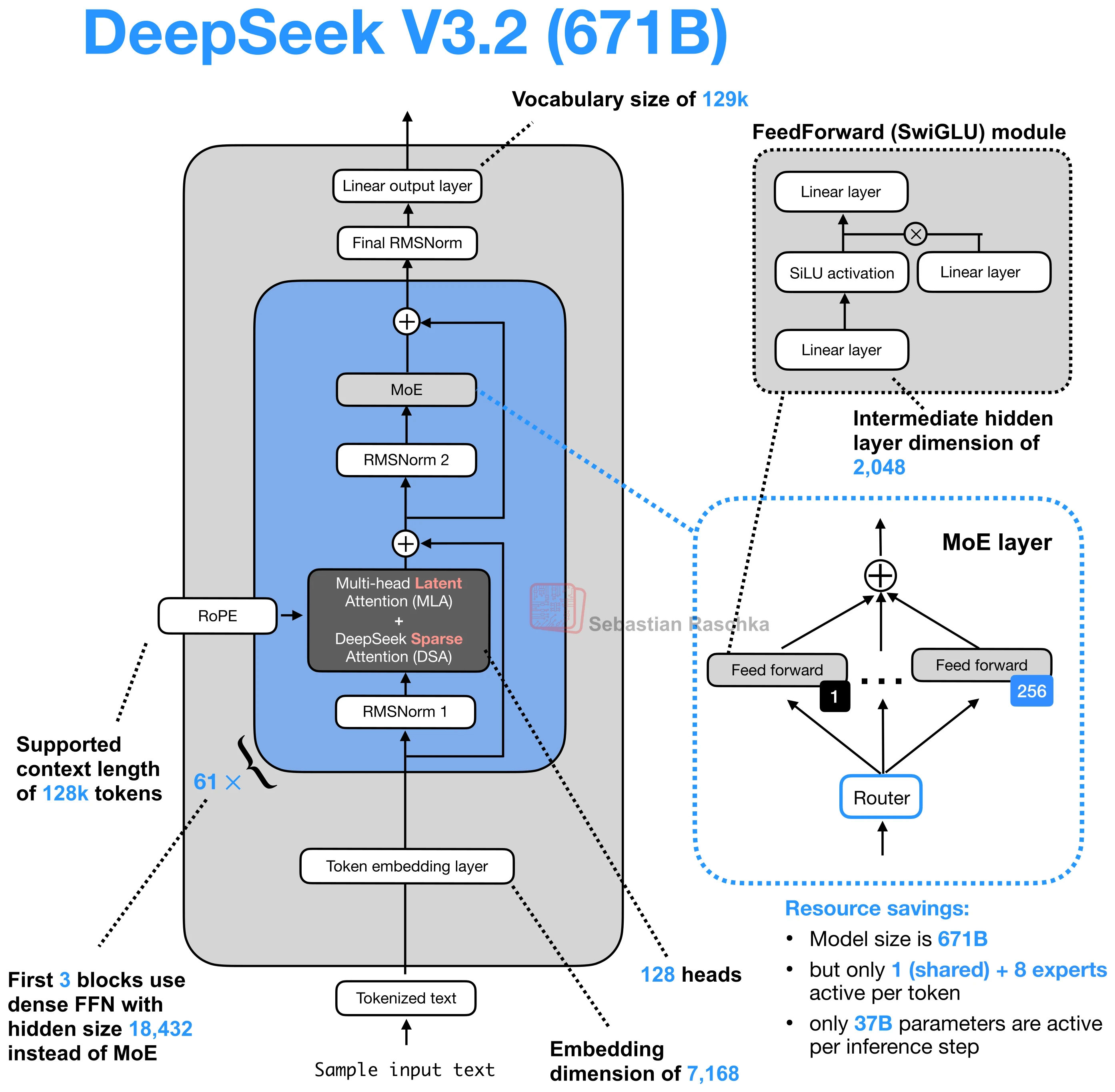
Figure 20: DeepSeek V3.2 is the obvious reference point, because this is the model family most closely associated with the sparse-attention idea.

The sparse pattern is not random. The first stage is a lightning indexer that scores previous tokens for each new query token. It uses MLA’s compressed token representations and computes a learned similarity score over the prior context, so the model can rank which earlier positions are worth revisiting.

The second stage is a token selector. It keeps only a smaller high-scoring subset, for example, a top-k set of past positions, and turns that subset into the sparse attention mask. So the main point is that DeepSeek Sparse Attention does not hard-code the sparsity pattern. It learns which past tokens to keep.
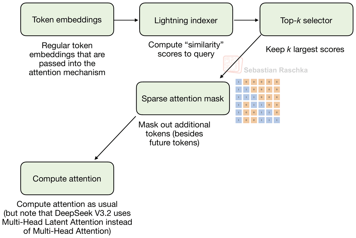
Figure 21: The mechanism consists of a lightning indexer that scores prior tokens and a selector that keeps only a smaller subset for attention (Original source: From DeepSeek V3 to V3.2: Architecture, Sparse Attention, and RL Updates).

DeepSeek Sparse Attention is relatively new and relatively complicated to implement, which is why it has not been so widely adopted as Grouped-Query Attention (GQA) yet.

6. Gated Attention

Gated attention is best understood as a modified full-attention block rather than as a separate attention family.

It usually appears inside hybrid stacks that still keep an occasional full-attention layer for exact content retrieval, but add a few stability-oriented changes on top of an otherwise familiar scaled dot-product attention block.
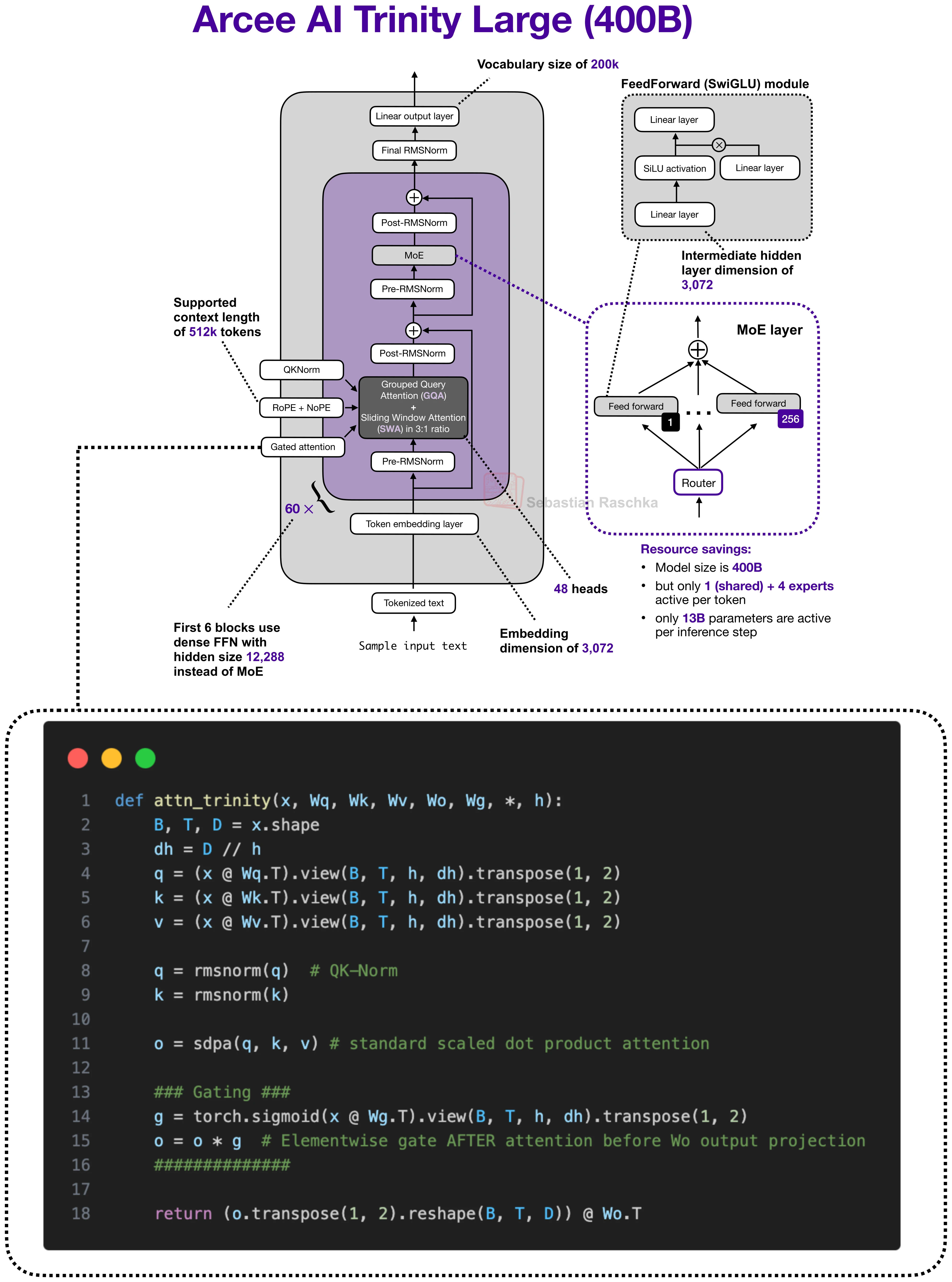
Figure 22: Trinity Large is a useful comparison because gated attention is not only a Qwen idea (more on that later). Here the gate appears after the scaled dot-product attention output and before the output projection in a different long-context architecture (Original source: A Dream of Spring for Open-Weight LLMs).

6.1 Where Gated Attention Appears

The Qwen3-Next and Qwen3.5 architectures show that recent hybrids (covered in the next section) do not replace attention everywhere. Instead, they replace most attention layers with a cheaper alternative and keep a smaller number of full-attention layers in the stack.

Those remaining full-attention layers are where gated attention typically appears. Qwen3-Next and Qwen3.5 use it together with Gated DeltaNet in a 3:1 pattern.

But hybrid architectures aside, Trinity uses a related gating idea in a more conventional attention stack, as shown in the previous figure above.

6.2 Gated Attention Relative To Standard Attention

The gated attention block in Qwen-style hybrids or Trinity (not a hybrid) is essentially standard scaled-dot-product attention with a few changes on top. In the original Gated Attention paper, those changes are presented as a way to make the retained full-attention layers behave more predictably inside a hybrid stack.

The block still looks like standard (full) attention, but it adds:

  1. an output gate that scales the attention result before it is added back to the residual,

  2. a zero-centered QK-Norm variant instead of standard RMSNorm for q and k,

  3. partial RoPE.

These are not changes on the scale of MLA or linear attention but merely stability and control changes applied to an otherwise familiar attention block.
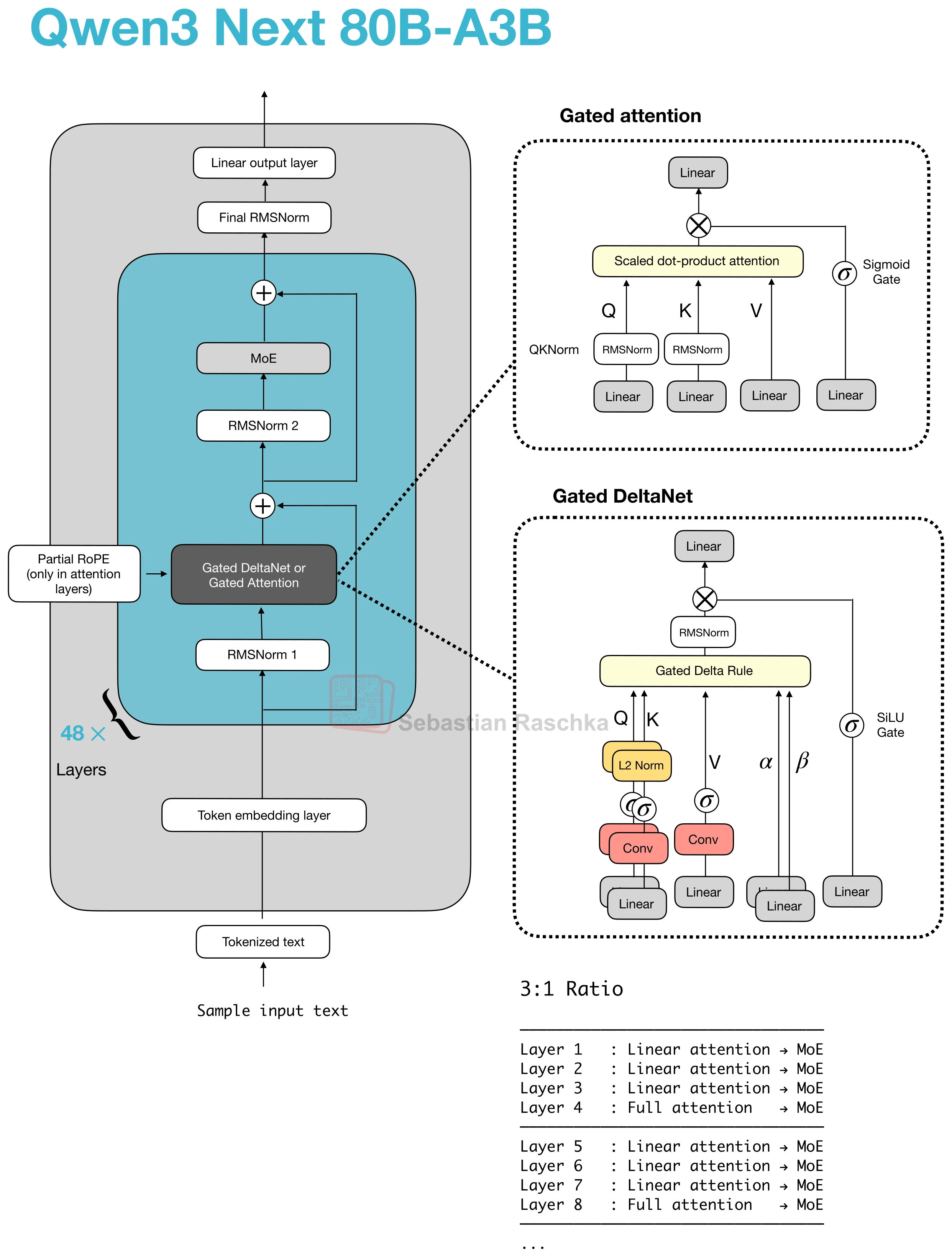
Figure 23: In Qwen3-Next and Qwen3.5, gated attention appears as the full-attention layer that periodically breaks up runs of Gated DeltaNet blocks.

Note that the figure above also includes Gated DeltaNet, which we will cover in the next section below.

7. Hybrid Attention

Hybrid attention is a broader design pattern rather than a specific, single mechanism. The overall idea is to keep a transformer-like stack, but replace most of the expensive full-attention layers with cheaper linear or state-space sequence modules.

The motivation is long-context efficiency. Full attention grows quadratically with sequence length, so once models move to contexts like 128k, 256k, or 1M tokens, attention memory and compute become expensive enough that using cheaper sequence modules in most layers while keeping only a smaller number of heavier retrieval layers starts making more sense. (Note that this comes with a bit of a modeling performance trade-off, though.)

In Qwen3-Next, this pattern appears as a 3:1 mix of Gated DeltaNet and Gated Attention blocks. Gated DeltaNet is also closely related to Mamba-2 (see the Gated Delta Networks: Improving Mamba2 with Delta Rule paper, for instance), and the mechanism can be read as a DeltaNet-style fast-weight update combined with Mamba-style gating. Later architectures keep the same overall idea but swap in other lightweight sequence mixers, such as Kimi Delta Attention, Lightning Attention, or standard Mamba-2.
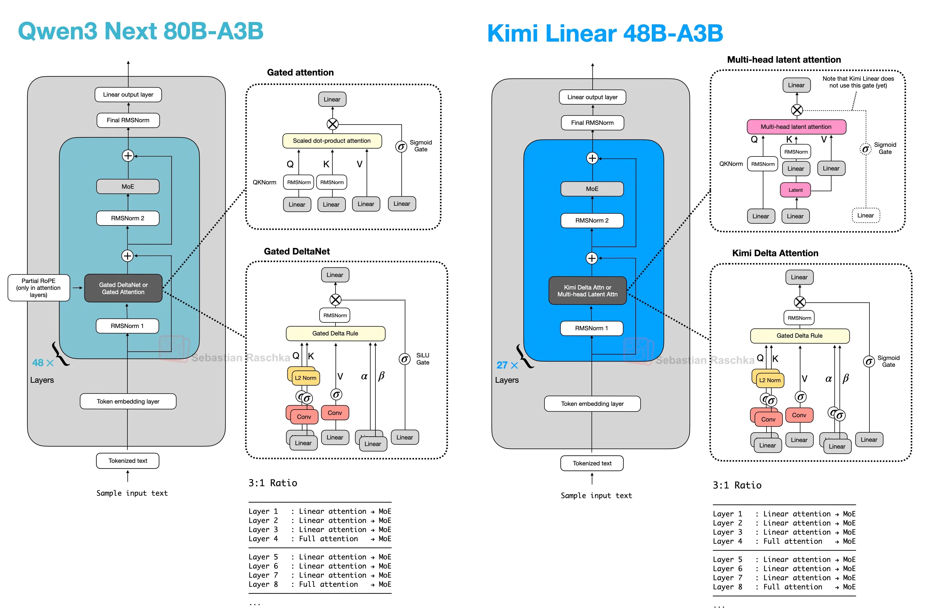
Figure 24: The basic hybrid pattern, where most blocks are cheaper sequence mixers and every fourth block restores a heavier attention layer (Original source The Big LLM Architecture Comparison).

7.1 Gated DeltaNet in Qwen3-Next

To my knowledge, the first prominent example of a close-to-flagship LLM with hybrid attention was Qwen3-Next in 2025, which does not remove attention completely but mixes three Gated DeltaNet blocks with one Gated Attention block.

Here, lightweight Gated DeltaNet blocks do most of the long-context work and keep memory growth much flatter than full attention. The heavier gated-attention layer remains because DeltaNet is less exact at content-based retrieval.

Inside a Gated DeltaNet block, the model computes query, key, and value vectors together with two learned gates (α, β). Rather than forming the usual token-to-token attention matrix, it writes to a small fast-weight memory using a delta-rule update. In rough terms, the memory stores a compressed running summary of past information, while the gates control how much new information is added and how much previous state is retained.

That makes Gated DeltaNet a linear-attention or recurrent-style mechanism rather than just another tweak to MHA. Relative to Mamba-2, the close connection is that both belong to the linear-time gated sequence-model family, but Gated DeltaNet uses a DeltaNet-style fast-weight memory update instead of the Mamba state-space update.
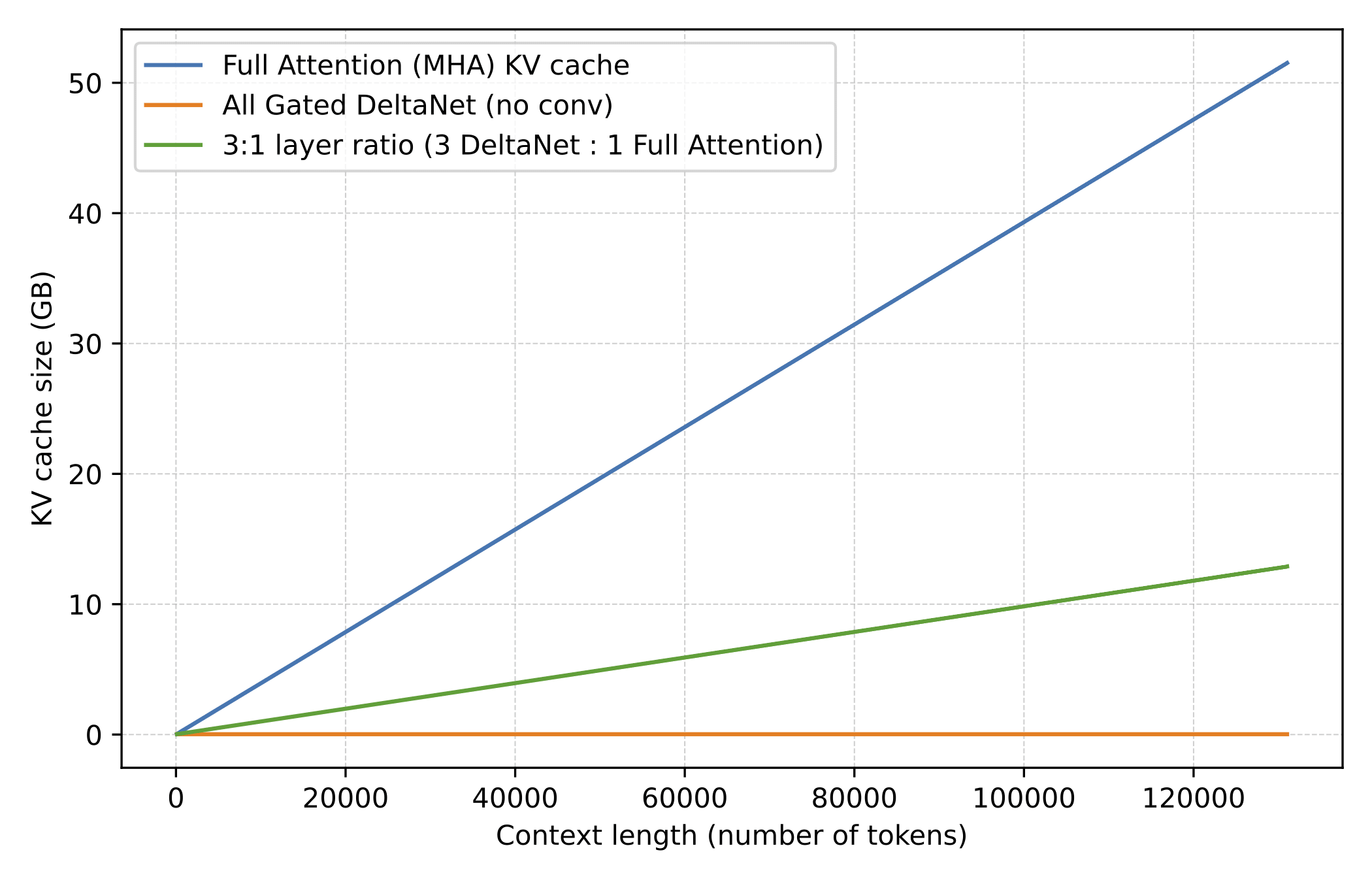
Figure 25: The practical motivation behind the hybrids is shown here in the memory curve. Hybrid stacks with Gated DeltaNet grow much more slowly with context length than ordinary full attention (Original source LLMs-from-scratch DeltaNet materials).

Qwen3.5 moves the former Qwen3-Next hybrid into Qwen’s main flagship series, which is an interesting move. This basically signals that the hybrid strategy is a success and that we may see more models with this architecture in the future.
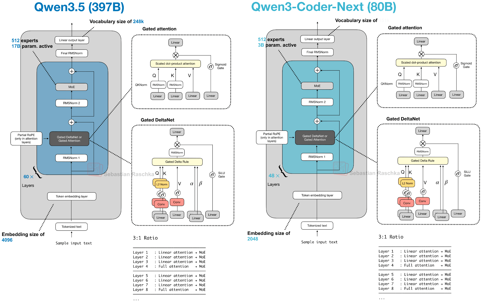
Figure 26: Qwen3.5 shows the Qwen team promoting the former Qwen3-Next side-branch into the main model line rather than leaving it as a one-off efficiency variant (Original source A Dream of Spring for Open-Weight LLMs).

7.2 Kimi Linear And Modified Delta Attention

Kimi Linear keeps the same broad transformer skeleton and the same 3:1 pattern, but it changes both halves of the recipe.

On the lightweight side, Kimi Delta Attention is a refinement of Gated DeltaNet. Where Qwen3-Next uses a scalar gate per head to control memory decay, Kimi uses channel-wise gating, which gives finer control over the memory update. On the heavier side, Kimi replaces Qwen3-Next’s gated-attention layers with gated MLA layers.

So, it’s still the same broader pattern as in Qwen3-Next and Qwen3.5, but both ingredients (slightly) change. I.e., most layers are still handled by a cheaper linear-style mechanism, and periodic heavier layers still remain for stronger retrieval.
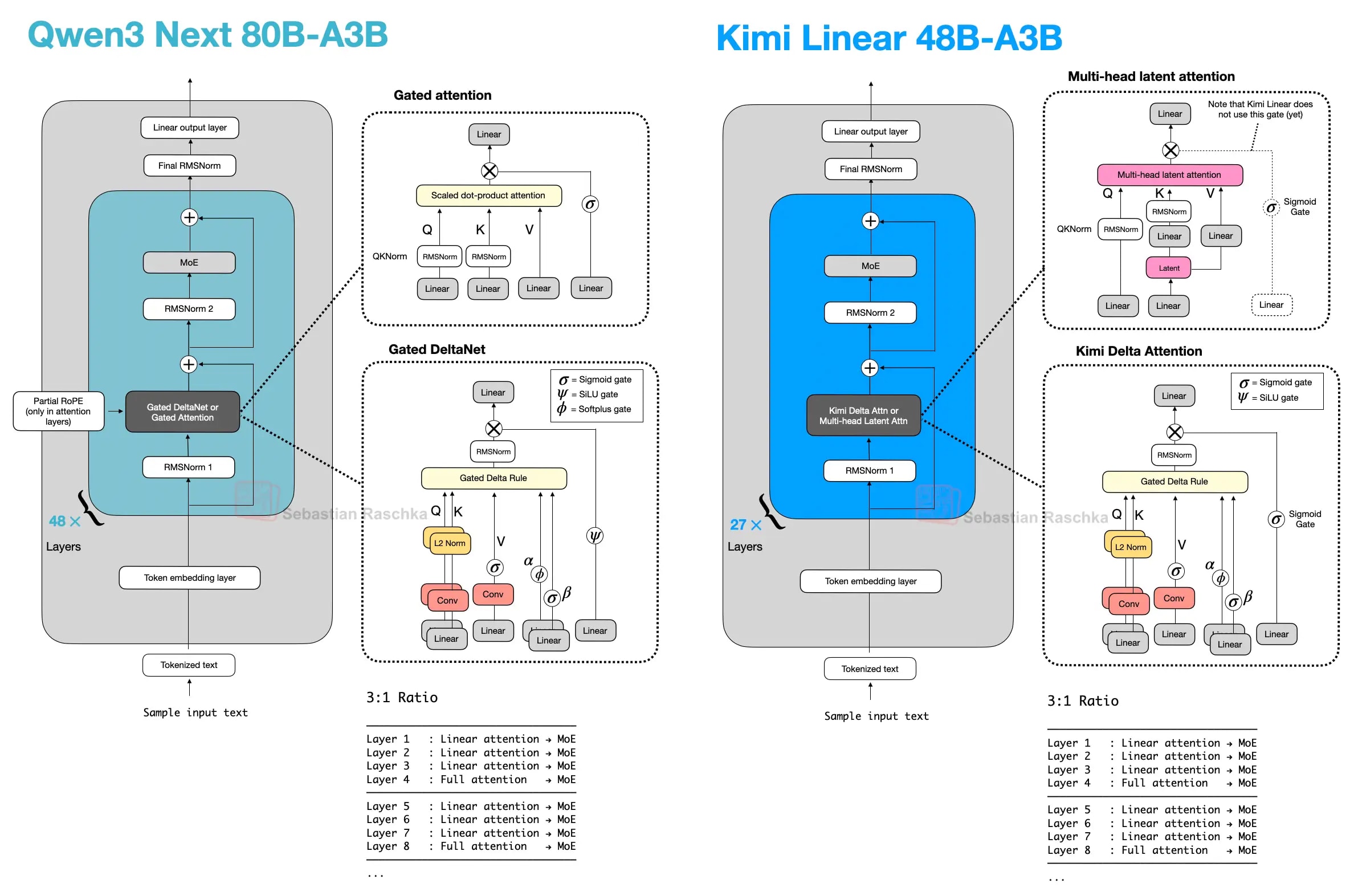
Figure 27: Kimi Linear keeps the same overall hybrid pattern while changing both the lightweight side and the heavier attention side of the stack (Original source The Big LLM Architecture Comparison).

7.3 Ling 2.5 And Lightning Attention

Ling 2.5 shows another swap on the lightweight side. Instead of Gated DeltaNet, Ling uses a slightly simpler recurrent linear attention variant called Lightning Attention. On the heavier side, it keeps MLA from DeepSeek.

Most sequence mixing happens in the cheaper linear-attention blocks, while a smaller number of heavier layers remain to preserve stronger retrieval. The difference is that the specific lightweight mechanism is now Lightning Attention rather than DeltaNet or Kimi Delta Attention.
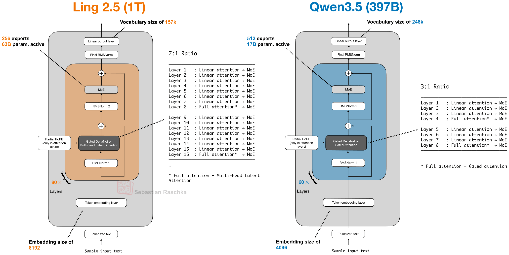
Figure 28: Ling 2.5 and Qwen3.5 are both linear-attention hybrids, even though Ling swaps in Lightning Attention and MLA instead of the Qwen recipe (Original source A Dream of Spring for Open-Weight LLMs).

Ling 2.5 is aimed more at long-context efficiency than at absolute benchmark leadership. According to the Ling team, it was reported as substantially faster than Kimi K2 at 32k tokens, which is the practical payoff these hybrids are aiming for.
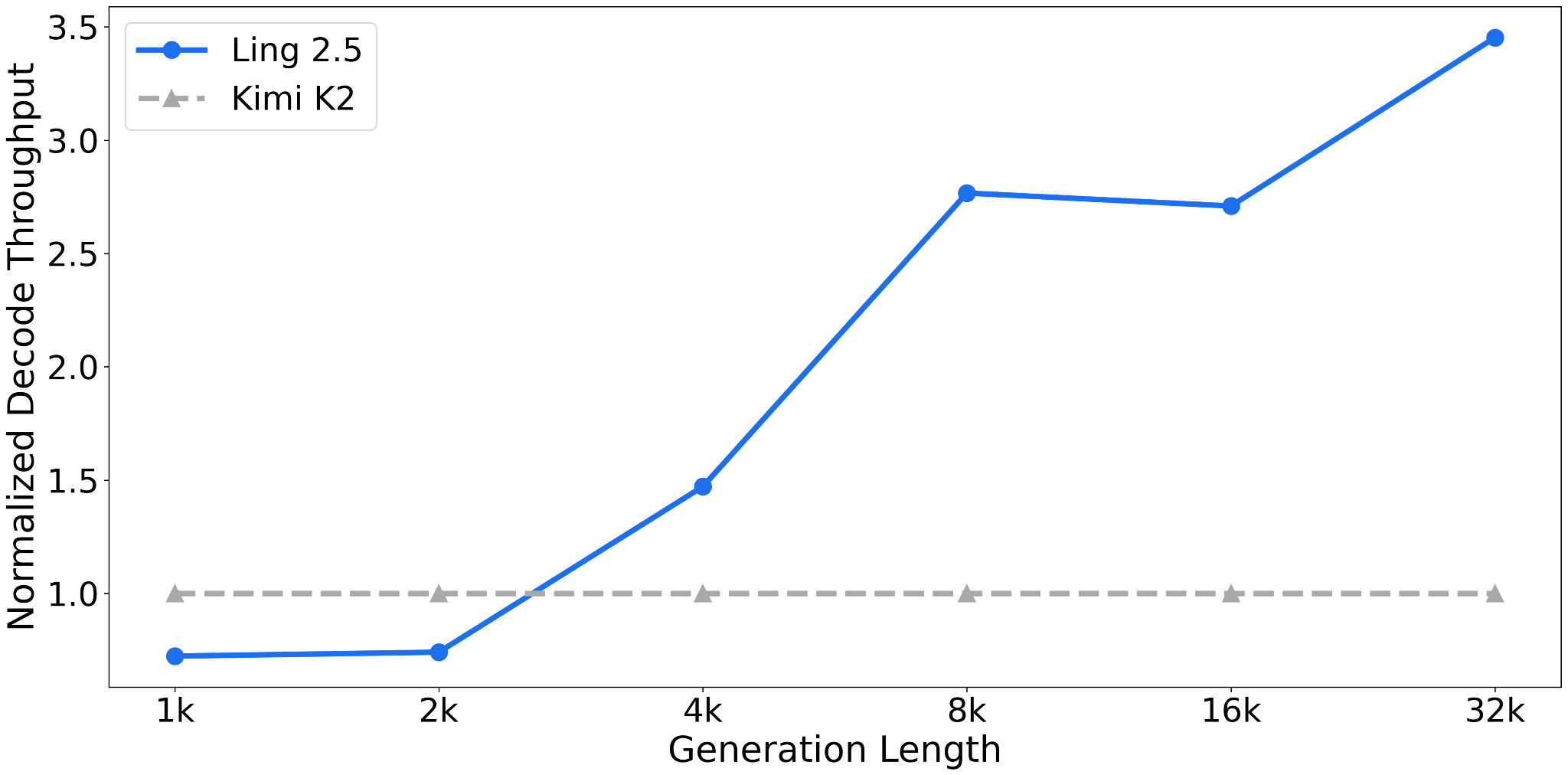
Figure 29: Ling 2.5 was presented as a strong efficiency upgrade, with much higher 32k-token throughput than Kimi K2 at the same 1-trillion-parameter scale (Original source Ling 2.5 model hub page).

Nemotron And Mamba-2

Nemotron pushes the pattern further away from the transformer baseline. Nemotron 3 Nano is a Mamba-Transformer hybrid that interleaves Mamba-2 sequence-modeling blocks with sparse MoE layers and uses self-attention only in a small subset of layers.

This is a more extreme version of the same basic tradeoff discussed above. Here, the lightweight sequence module is a Mamba-2 state-space block rather than a DeltaNet-style fast-weight update, but the basic tradeoff is similar.
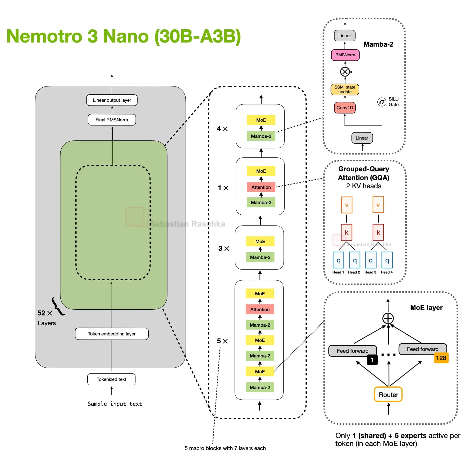
Figure 30: Nemotron 3 Nano uses Mamba-2 for most of the sequence modeling work, with self-attention only appearing in a small subset of layers (Original source The Big LLM Architecture Comparison).

The larger Nemotron 3 Super keeps the Mamba-2 hybrid attention approach and adds other efficiency-oriented changes such as latent MoE and shared-weight multi-token prediction (MTP) for speculative decoding.
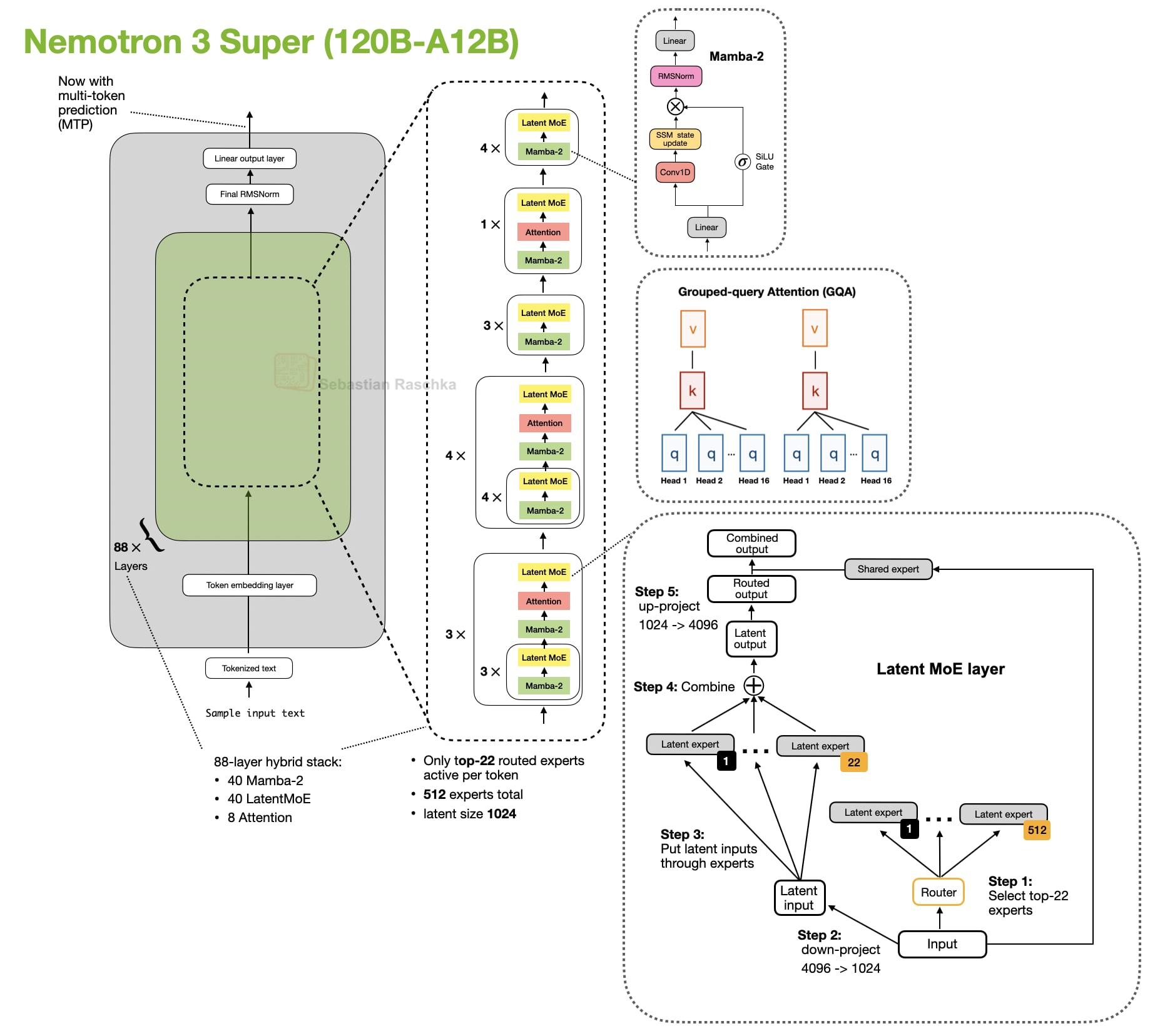
Figure 31: Nemotron 3 Super keeps the Mamba-2 hybrid attention pattern while adding latent MoE and shared-weight MTP on top (Original source The Big LLM Architecture Comparison).

Conclusion

Of course, there are many more (mostly niche) attention variants throughout the literature that I haven’t covered here. The focus of this article was on those that are currently used in state-of-the-art (open-weight) models.

In particular, I am looking forward to (1) seeing the brand new Mamba-3 layers getting integrated into the aforementioned hybrid architectures (replacing Gated DeltaNet) and (2) attention residuals being used in general.

In practice, you may also wonder what the “best” architecture is at the moment. This is hard to answer, as there are no public experiments that train different architectures on the same training data etc.

Hence, we can currently only answer what the best (trained) model choice is for a given problem. In my opinion, hybrid architectures are still a novelty, and the main selling point is mainly (long-context) efficiency versus just modeling performance. Hence, I think they are a great candidate for agent contexts (like OpenClaw).

Personally, I think the problem with hybrid architectures is also that the inference stacks are not quite as optimized, yet, and I find that I get better tok/sec throughput when running LLMs locally using more classic setups like GPT-OSS with grouped-query attention.

Anyways, I am curious to see what DeepSeek V4 has in store, since DeepSeek has been quite the reliable trend-setter in the recent 2 years.

A Dream of Spring for Open-Weight LLMs: 10 Architectures from Jan-Feb 2026

25 February 2026 at 13:26

If you have struggled a bit to keep up with open-weight model releases this month, this article should catch you up on the main themes.

In this article, I will walk you through the ten main releases in chronological order, with a focus on the architecture similarities and differences:

  1. Arcee AI’s Trinity Large (Jan 27, 2026)

  2. Moonshot AI’s Kimi K2.5 (Jan 27, 2026)

  3. StepFun Step 3.5 Flash (Feb 1, 2026)

  4. Qwen3-Coder-Next (Feb 3, 2026)

  5. z.AI’s GLM-5 (Feb 12, 2026)

  6. MiniMax M2.5 (Feb 12, 2026)

  7. Nanbeige 4.1 3B (Feb 13, 2026)

  8. Qwen 3.5 (Feb 15, 2026)

  9. Ant Group’s Ling 2.5 1T & Ring 2.5 1T (Feb 16, 2026)

  10. Cohere’s Tiny Aya (Feb 17, 2026)

  11. Update 1: Sarvam 30B and 105B (Mar 6, 2026)

(PS: DeepSeek V4 will be added once released.)

Since there’s a lot of ground to cover, I will be referencing my previous The Big LLM Architecture Comparison article for certain technical topics (like Mixture-of-Experts, QK-Norm, Multi-head Latent Attention, etc.) throughout this article for background information to avoid redundancy in this article.

1. Arcee AI’s Trinity Large: A New US-Based Start-Up Sharing Open-Weight Models

On January 27, Arcee AI (a company I hadn’t had on my radar up to then) began releasing versions of their open-weight 400B Trinity Large LLMs on the model hub, along with two smaller variants:

  • Their flagship large model is a 400B param Mixture-of-Experts (MoE) with 13B active parameters.
  • The two smaller variants are Trinity Mini (26B with 3B active parameters) and Trinity Nano (6B with 1B active parameters).

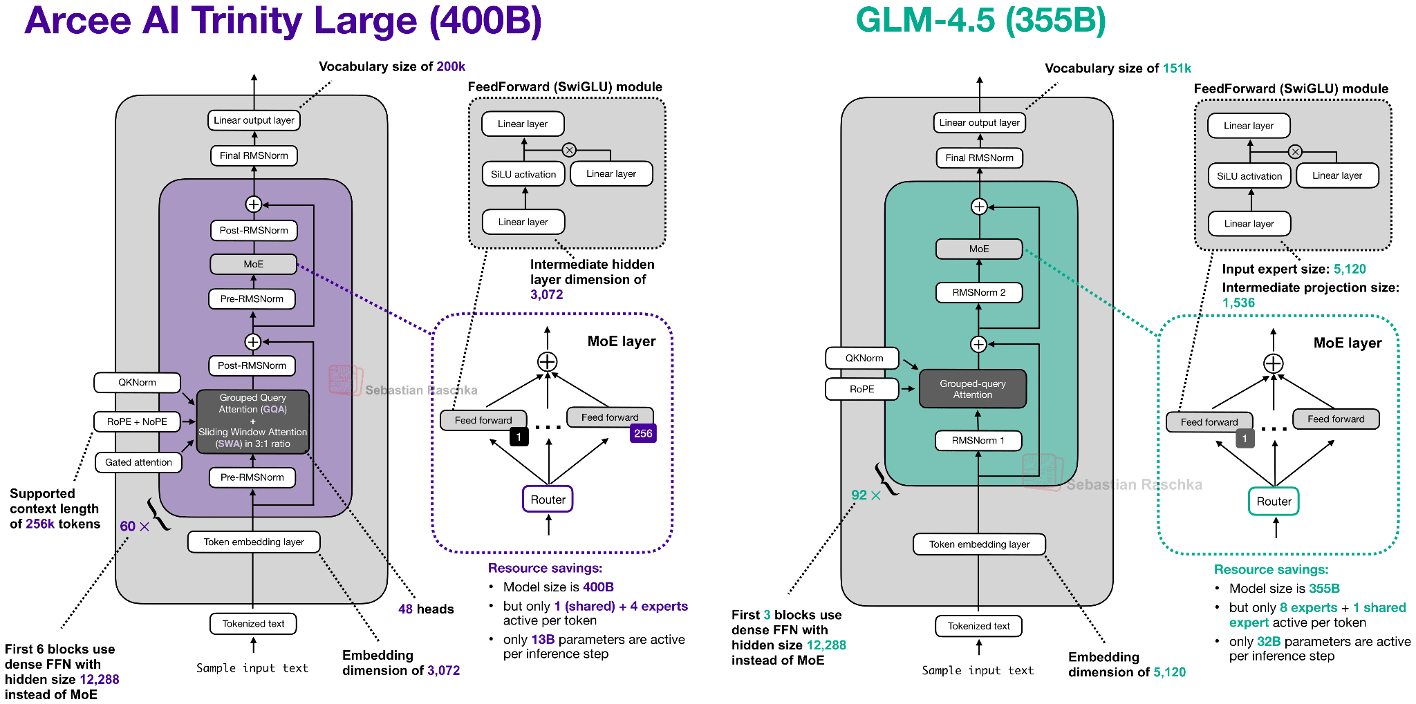
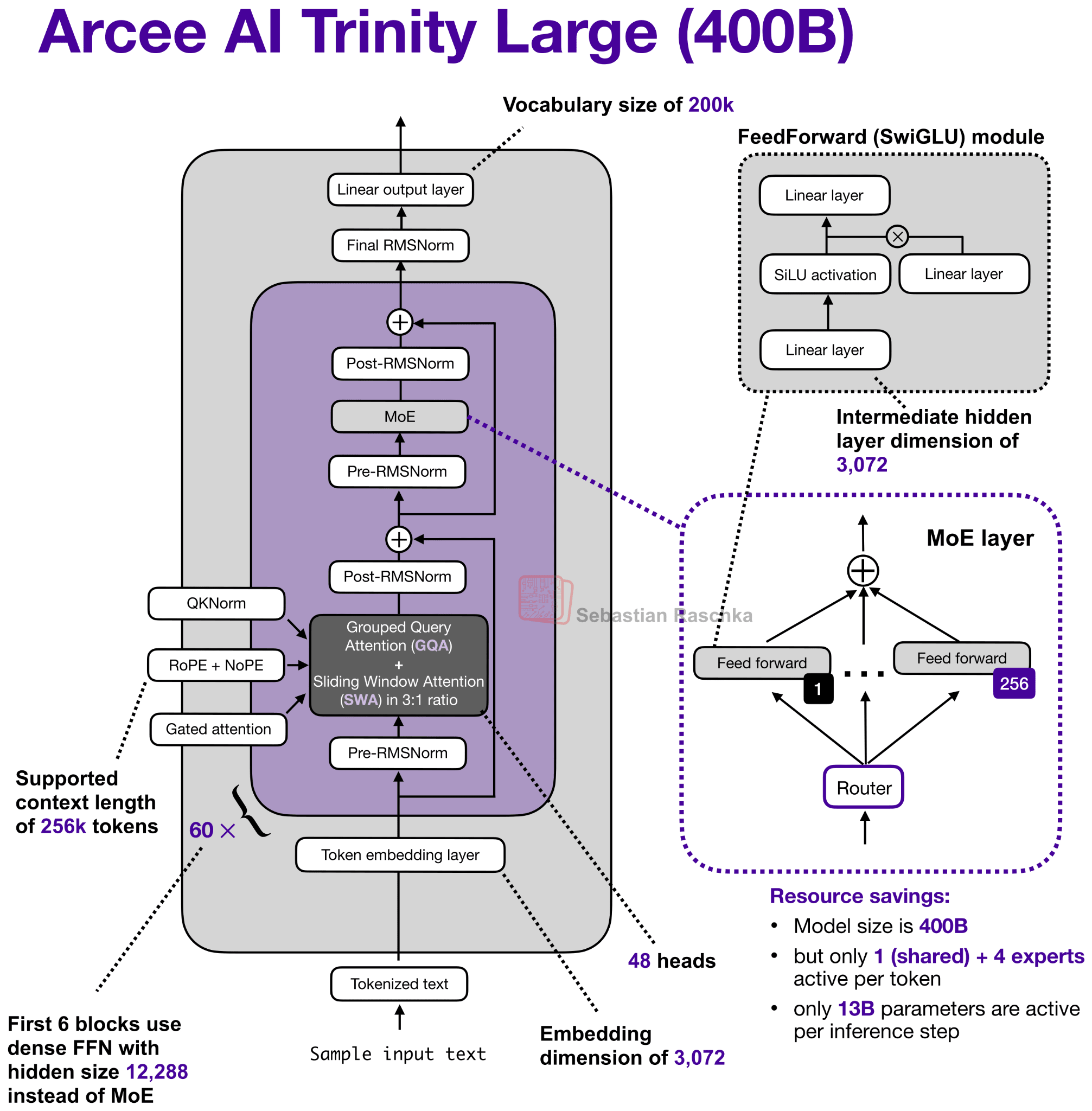
Figure 1: Overview of the Trinity Large architecture (based on the model hub config file).

Along with the model weights, Arcee AI also released a nice technical report on GitHub (as of Feb 18 also on arxiv) with lots of details.
So, let’s take a closer look at the 400B flagship model. Figure 2 below compares it to z.AI’s GLM-4.5, which is perhaps the most similar model due to its size with 355B parameters.
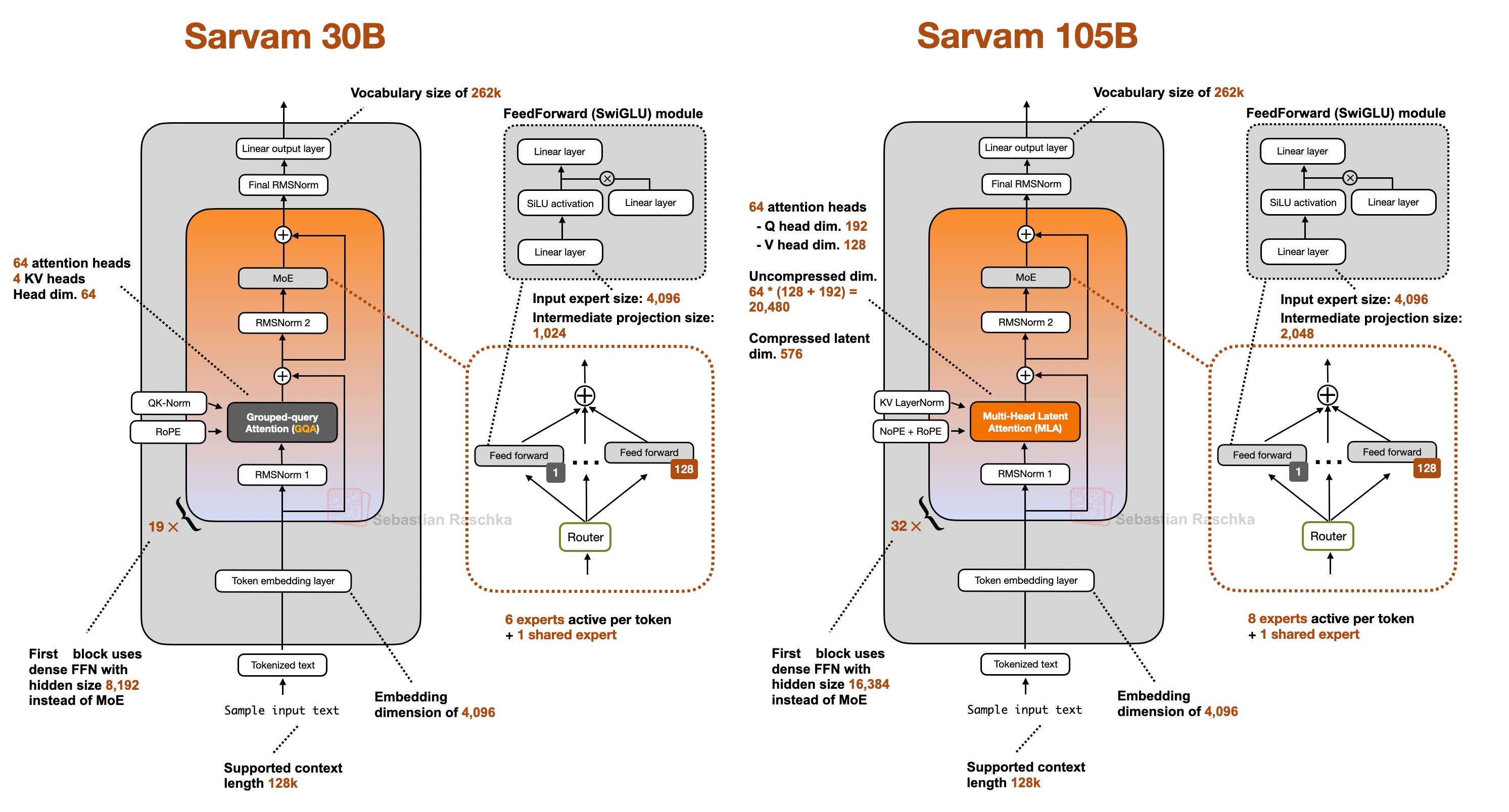
Figure 2: Arcee AI Trinity Large next to GLM-4.5 of a relatively similar size (400B vs 355B).

As we can see in the Trinity and GLM-4.5 comparison, there are several interesting architectural components added to the Trinity model.

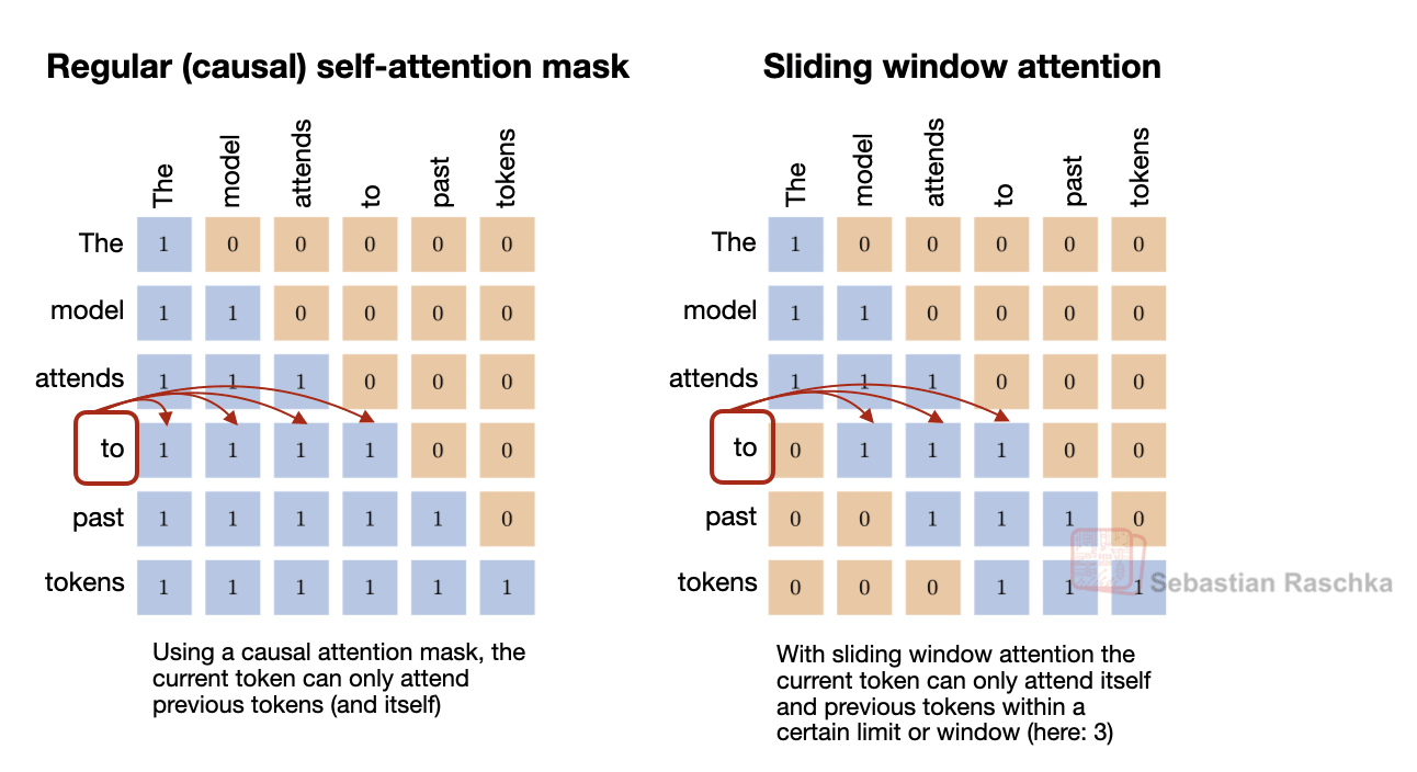
First, there are the alternating local:global (sliding window) attention layers (SWA) like in Gemma 3, Olmo 3, Xiaomi MiMo, etc. In short, SWA is a type of sparse (local) attention pattern where each token attends only to a fixed-size window of t recent tokens (for example, 4096) instead of attending to the entire input (which could be up to n=256,000 tokens). This reduces the per-layer regular attention cost from O(n²) to roughly O(n·t) for sequence length n, which is why it is attractive for long-context models.

Figure 3: A comparison between regular attention (global attention) and sliding window attention (local attention).

But instead of using the common 5:1 local:global ratio that Gemma 3 and Xiaomi used, the Arcee team opted for a 3:1 ratio similar to Olmo 3, and a relatively large sliding window size of 4096 (also similar to Olmo 3).

The architecture also uses QK-Norm, which is a technique that applies RMSNorm to the keys and queries to stabilize training (as shown in Figure 4 below), as well as no positional embeddings (NoPE) in the global attention layers similar to SmolLM3.

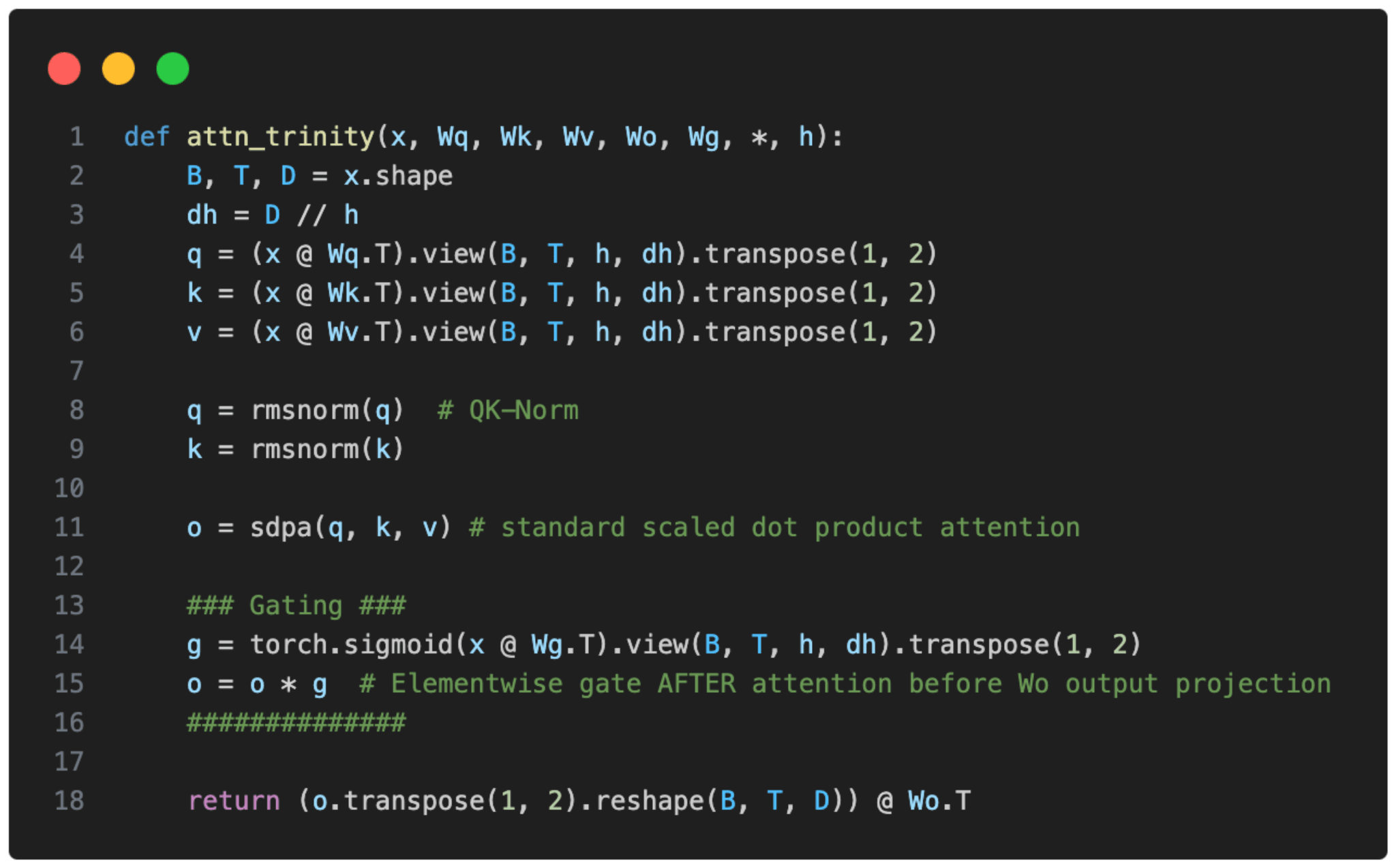
Trinity also has a form of gated attention. It’s not a full-blown Gated DeltaNet but it uses a similar gating as in the attention mechanism in Qwen3-Next.

I.e., the Trinity team modified the standard attention by adding elementwise gating to the scaled dot-product before the output linear projection (as shown in the figure below), which reduces attention sinks and improves long-sequence generalization. Additionally, it also helped with training stability.

Figure 4: Illustration of the gating mechanism that Trinity Large uses in the attention mechanism.

Also, the Trinity technical report showed that the modeling performance of the Trinity Large and GLM-4.5 base models are practically identical (I assume they didn’t compare it to more recent base models because many companies only share their fine-tuned models these days.)

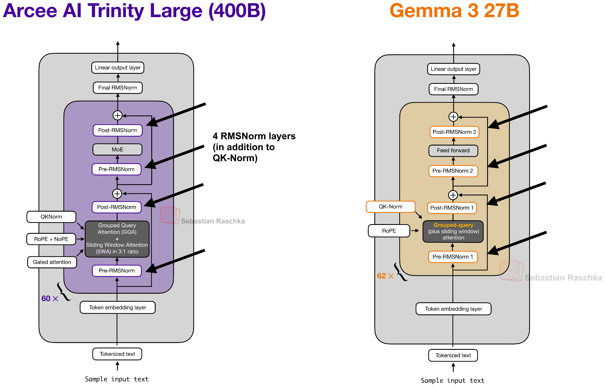
You may have noticed the use of four (instead of two) RMSNorm layers in the previous Trinity Large architecture figure which looks similar to Gemma 3 at first glance.

Figure 5: Arcee Trinity and Gemma 3 RMSNorm placement side by side.

Overall, the RMSNorm placement looks like a Gemma 3-like RMSNorm placement, but the twist here is that the gain of the second RMSNorm (in each block) is depth-scaled, meaning it’s initialized to about 1 / sqrt(L) (with L the total number of layers). So, early in training, the residual update starts small and grows as the model learns the right scale.

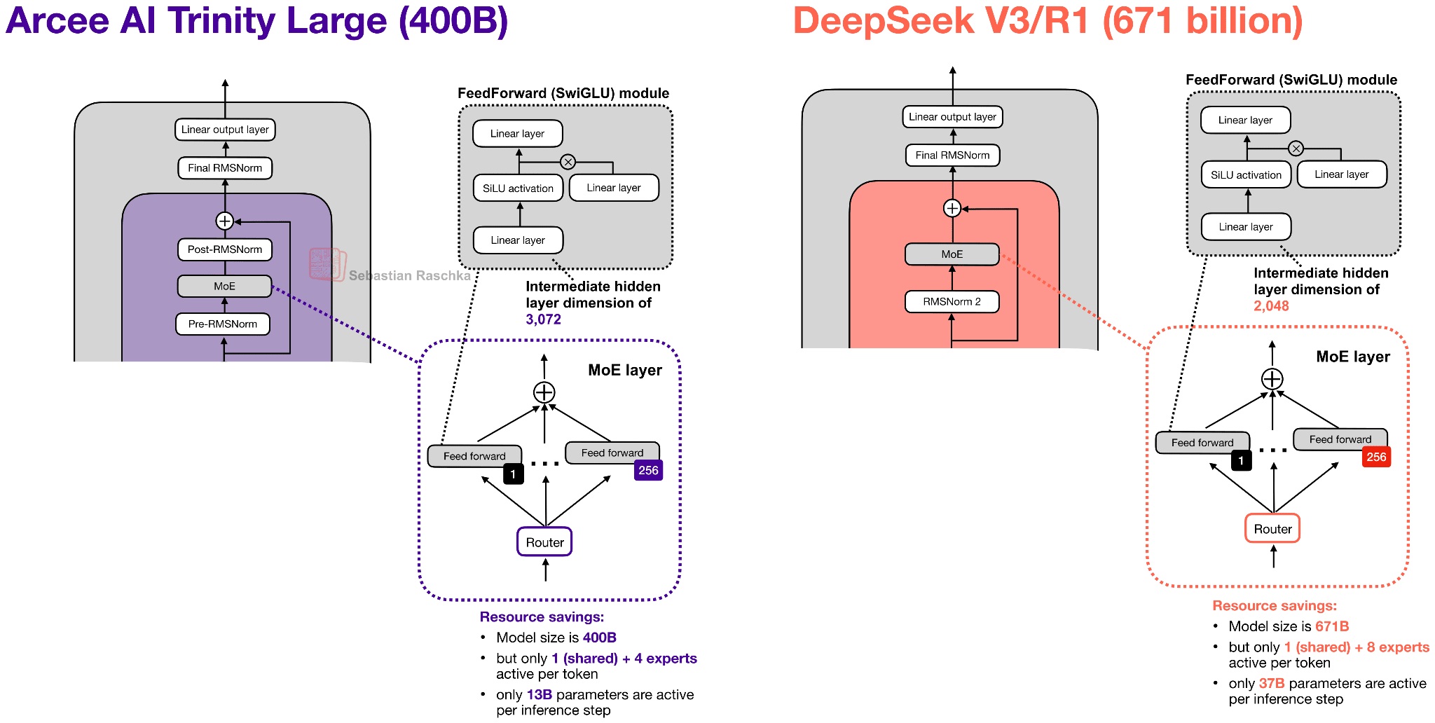
Figure 6: Arcee Trinity and DeepSeek V3/R1 MoE side by side.

The MoE is a DeepSeek-like MoE with lots of small experts, but made it coarser as that helps with inference throughput (something we have also seen in Mistral 3 Large when they adopted the DeepSeek V3 architecture).

Lastly, there are some interesting details on the training improvements (a new MoE load-balancing strategy and another using the MuOpt optimizer), but since this is a mainly an architecture article (and there are many more open-weight LLMs to cover), these details are out of scope.

2. Moonshot AI’s Kimi K2.5: A DeepSeek-Like Model at a 1-Trillion-Parameter Scale

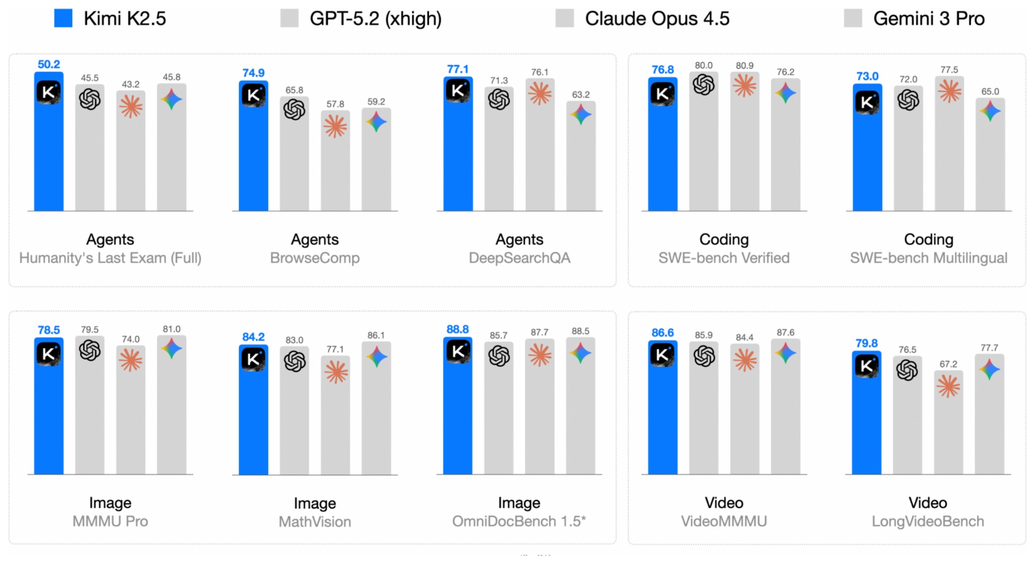
While Arcee Trinity essentially matched the modeling performance of the older GLM-4.5 model, Kimi K2.5 is an open-weight model that set a new open-weight performance ceiling at the time of its release on Jan 27.

​Impressively, according to their own benchmarks in their detailed technical report, it was on par with the leading proprietary models at the time of its release.

​

Figure 7: Kimi K2.5 performance benchmark from the official K2.5 technical report.

The good modeling performance is no surprise when compared to, e.g., Arcee Trinity or GLM-4.5 covered earlier, since (similar to its K2 predecessor), Kimi K2.5 is a 1-trillion-parameter model and thus 2.5x larger than Trinity and 2.8x larger than GLM-4.5.

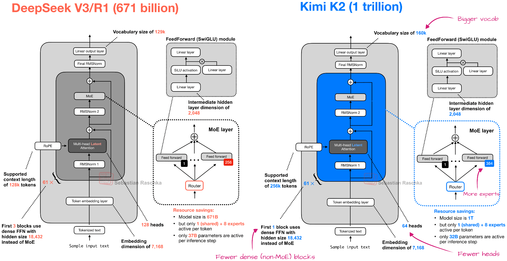
Overall, the Kimi K2.5 architecture is similar to Kimi K2, which, in turn, is a scaled-up version of the DeepSeek V3 architecture.

Figure 8: Kimi K2 is a larger version of the DeepSeek V3 architecture.

However, K2 was a pure text model, and Kimi K2.5 is now a multimodal model with vision support. To quote from the technical report:

​> Kimi K2.5 is a native multimodal model built upon Kimi K2 through large-scale joint pre-training on approximately 15 trillion mixed visual and text tokens.

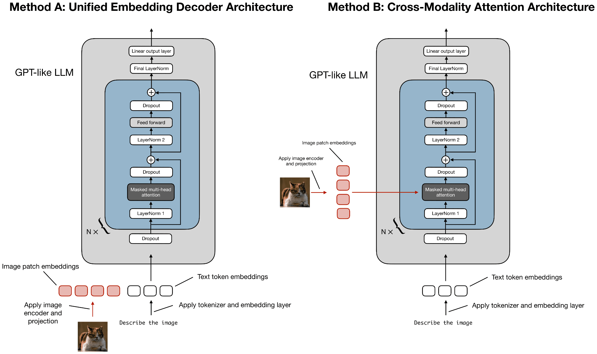
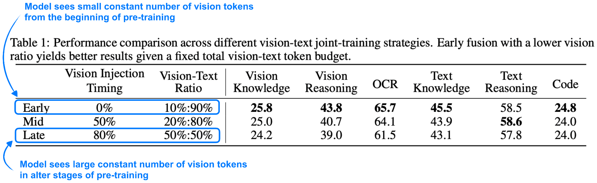
During the training, they adopted an early fusion approach and passed in the vision tokens early on alongside the text tokens, as I discussed in my older Understanding Multimodal LLMs article.

Figure 9: Like most other contemporary multimodal LLMs, Kimi K2.5 uses method A, passing the vision tokens alongside the text tokens during training.

Side note: In multimodal papers, “early fusion” is unfortunately overloaded. It can mean either

1. When the model sees vision tokens during pre-training. I.e., vision tokens are mixed in from the start (or very early) of pre-training as opposed to later stages.

2. How the image tokens are combined in the model. I.e., they are fed as embedded tokens alongside the text tokens.

In this case, while the term “early fusion” in the report specifically refers to point 1 (when the vision tokens are provided during pre-training), point 2 is also true here.

Furthermore, regarding point 1, the researchers included an interesting ablation study showing that the model benefits from seeing vision tokens early in pre-training, as shown in the annotated table below.

Figure 10: Given a fixed number of vision tokens during training, the model performance benefits if the model is shown a smaller number of vision tokens early on during pre-training (as opposed to adding a higher number of vision tokens later on). Annotated table from the Kimi K2.5 technical report.

3. StepFun’s Step 3.5 Flash: Good Performance at Great Tokens/Sec Throughput

I have to admit that I haven’t had the Step models on my radar yet. This one caught my attention due to its interesting size, detailed technical report, and fast tokens/sec performance.

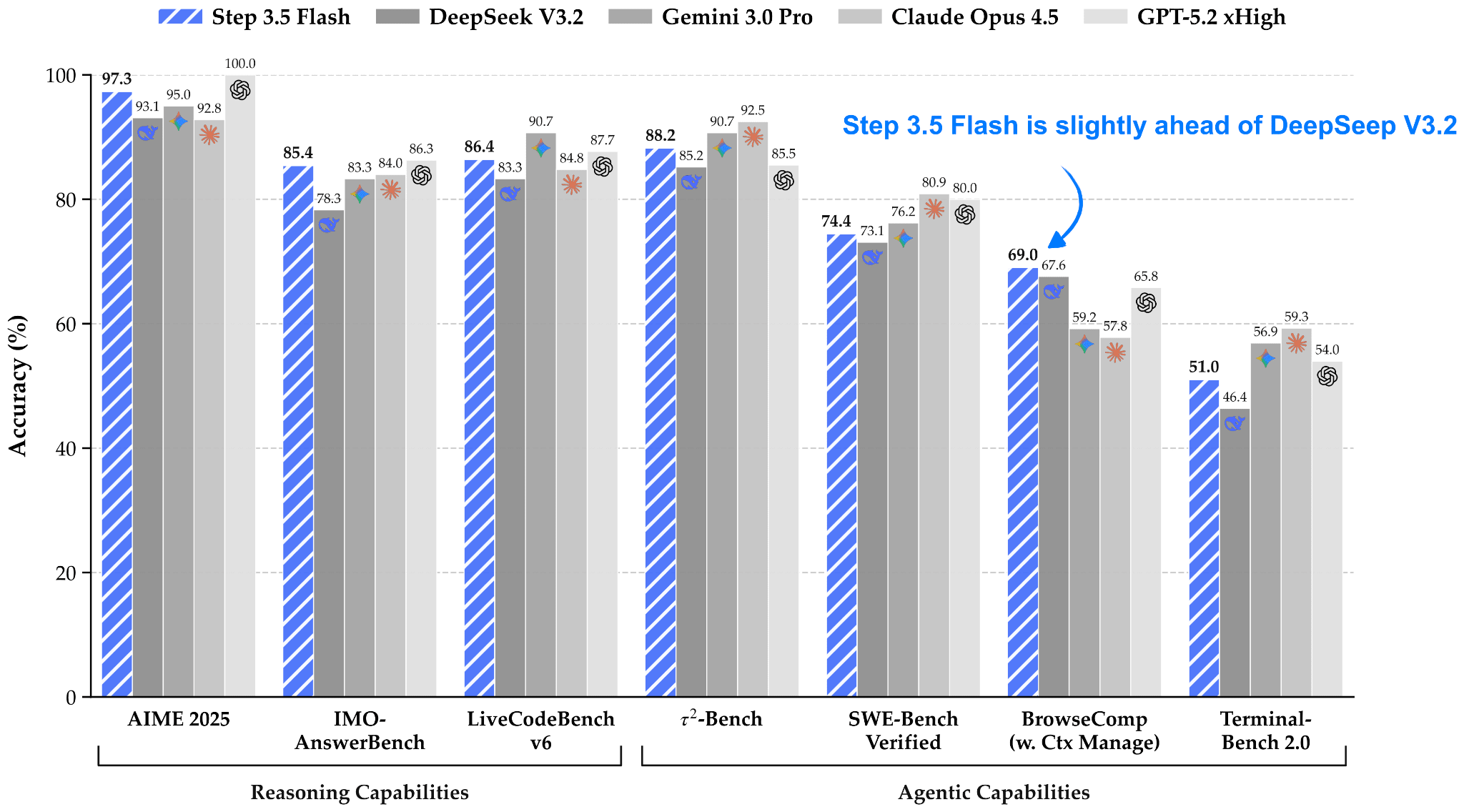
Step 3.5 Flash is a 196B parameter model that is more than 3x smaller than the recent DeepSeek V3.2 model (671B) while being slightly ahead in modeling performance benchmarks. According to the Step team, Step 3.5 Flash has a 100 tokens/sec throughput at a 128k context length, whereas DeepSeek V3.2 has only a 33 tokens/sec throughput on Hopper GPUs, according to the data on the Step model hub page.

Figure 11: Step 3.5 Flash benchmark from the Step technical report.

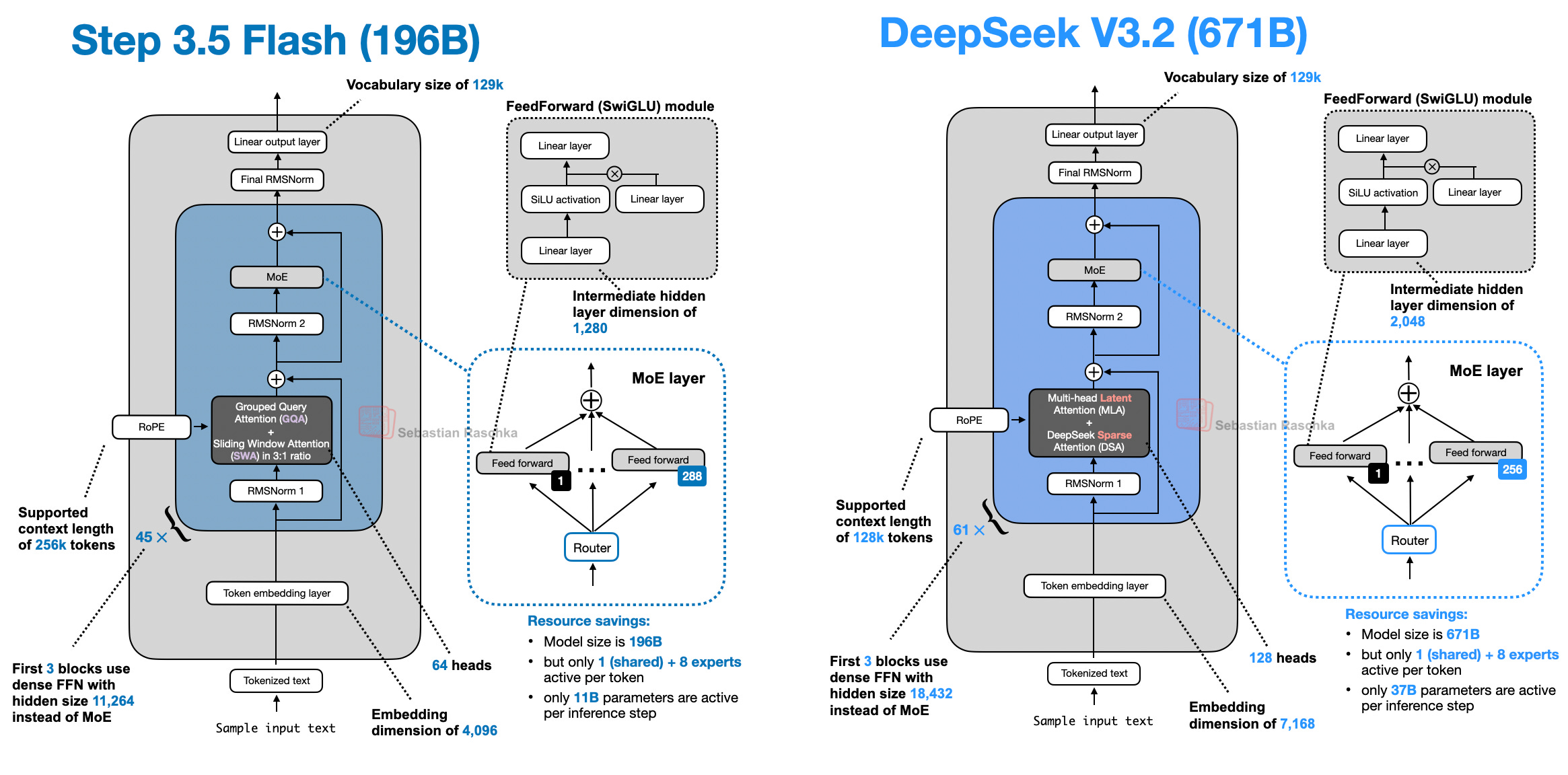
One reason for this higher performance is the model’s smaller size (196B-parameter MoE with 11B parameters active per token versus 671B-parameter MoE with 37B parameters active), as shown in the figure below.

Figure 12: Step 3.5 Flash and DeepSeek V3.2 side by side.

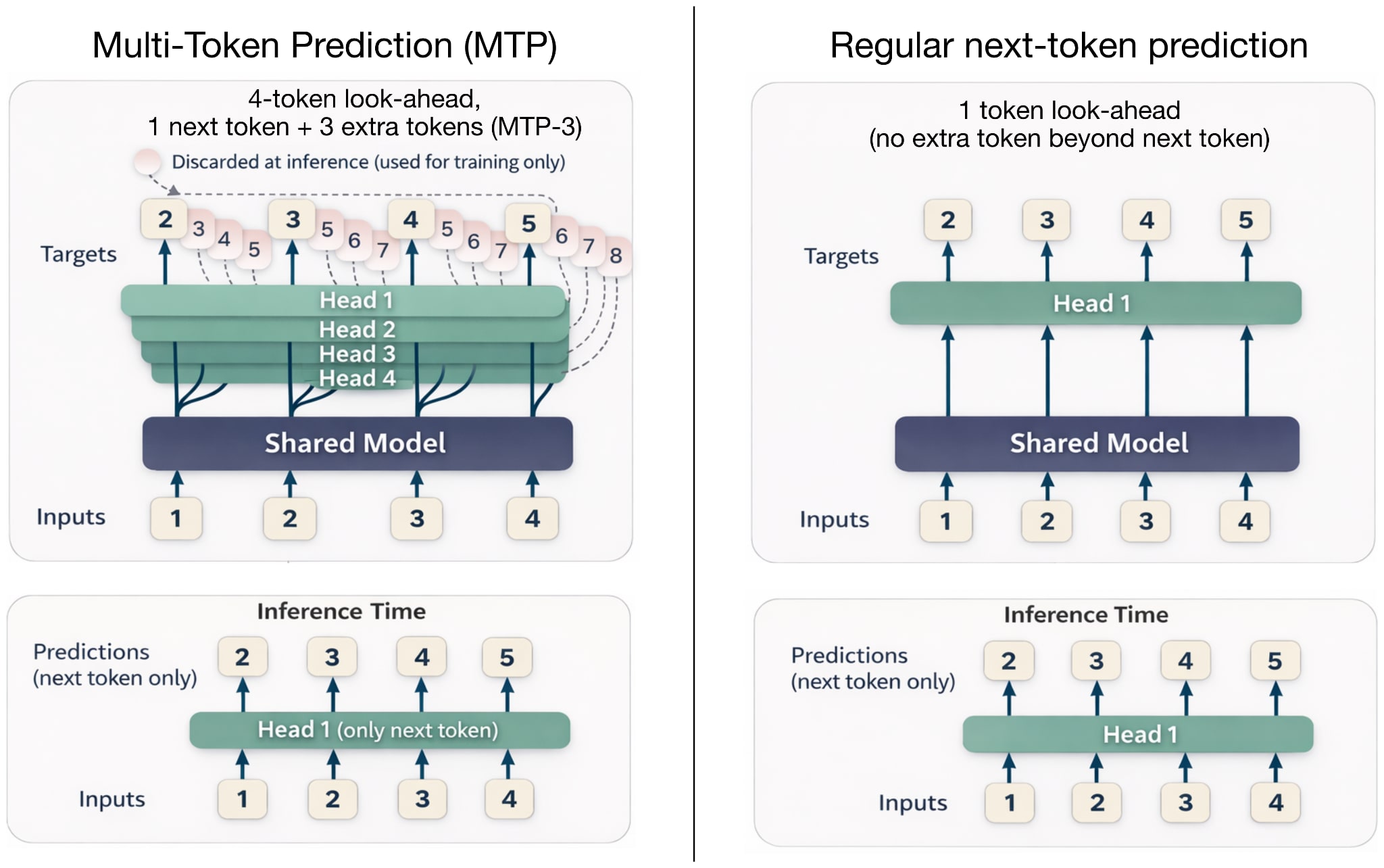
The other reason along with gated attention (which we previously discussed in the context of Trinity) is Multi-Token Prediction (MTP). DeepSeek has been an early adopter of multi-token prediction, a technique that trains the LLM to predict multiple future tokens at each step, rather than a single one. Here, at each position t, small extra heads (linear layers) output logits for t+1...t+k, and we sum cross-entropy losses for these offsets (in the MTP paper, the researchers recommended k=4).

This additional signal speeds up training, and inference may remain at generating one token at a time, as illustrated in the figure below.

Figure 13: Multi-Token Prediction versus regular next token prediction. (Left subfigure inspired by the MTP paper.) Originally, MTP was only used during training, not inference; hence, the inference time steps (bottom) show a single next-token prediction.

DeepSeek V3 reported using MTP-1, that is, MTP with 1 extra token (instead of 3) during training, and then making MTP optional during inference.

Step 3.5 Flash uses MTP with 3 additional tokens (MTP-3) during both training and inference (note that MTP is usually not used during inference, and this is an exception).

​Note that the previously discussed Arcee Trinity and Kimi K2.5 do not use MTP, but other architectures already use an MTP-3 setup similar to Step 3.5 Flash, for example, GLM-4.7 and MiniMax M2.1.

4. Qwen3-Coder-Next: An Attention-Hybrid for Coding

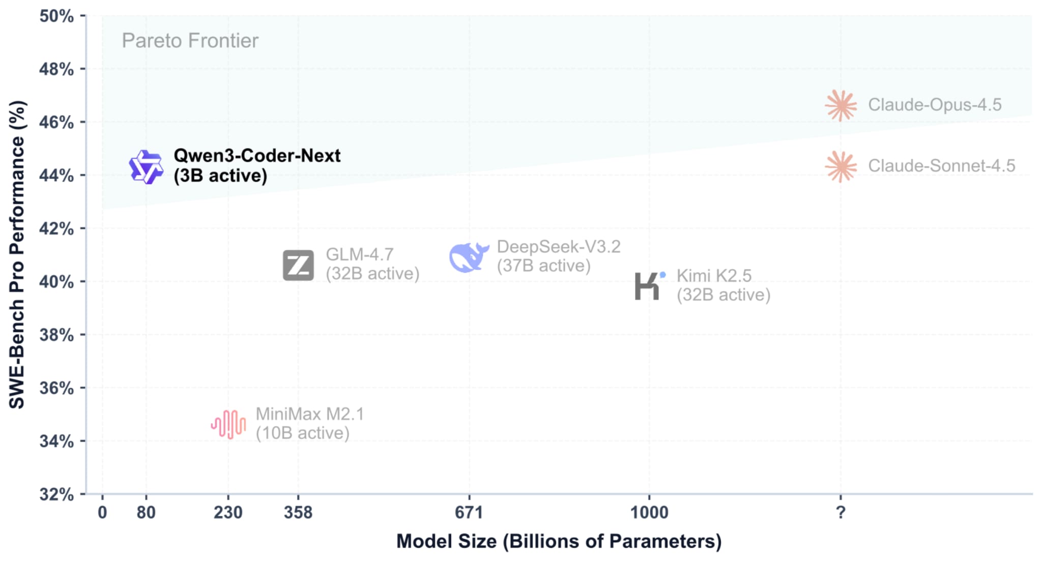
In early February 2026, the Qwen3 team shared the 80B Qwen3-Coder-Next model (3B parameters active), which made big headlines for outperforming much larger models like DeepSeek V3.2 (37B active) and Kimi K2.5 and GLM-4.7 (both 32B active) on coding tasks.

Figure 14: Qwen3-Coder-Next performance on a coding benchmark next to other popular coding models; this figure appeared in the official technical report.

Moreover, as shown in the benchmark figure above, the Qwen3-Coder-Next SWE-Bench Pro performance is roughly on par with Claude Sonnet 4.5 (and only slightly below Claude Opus 4.5), which is impressive for a relatively small open-weight model!

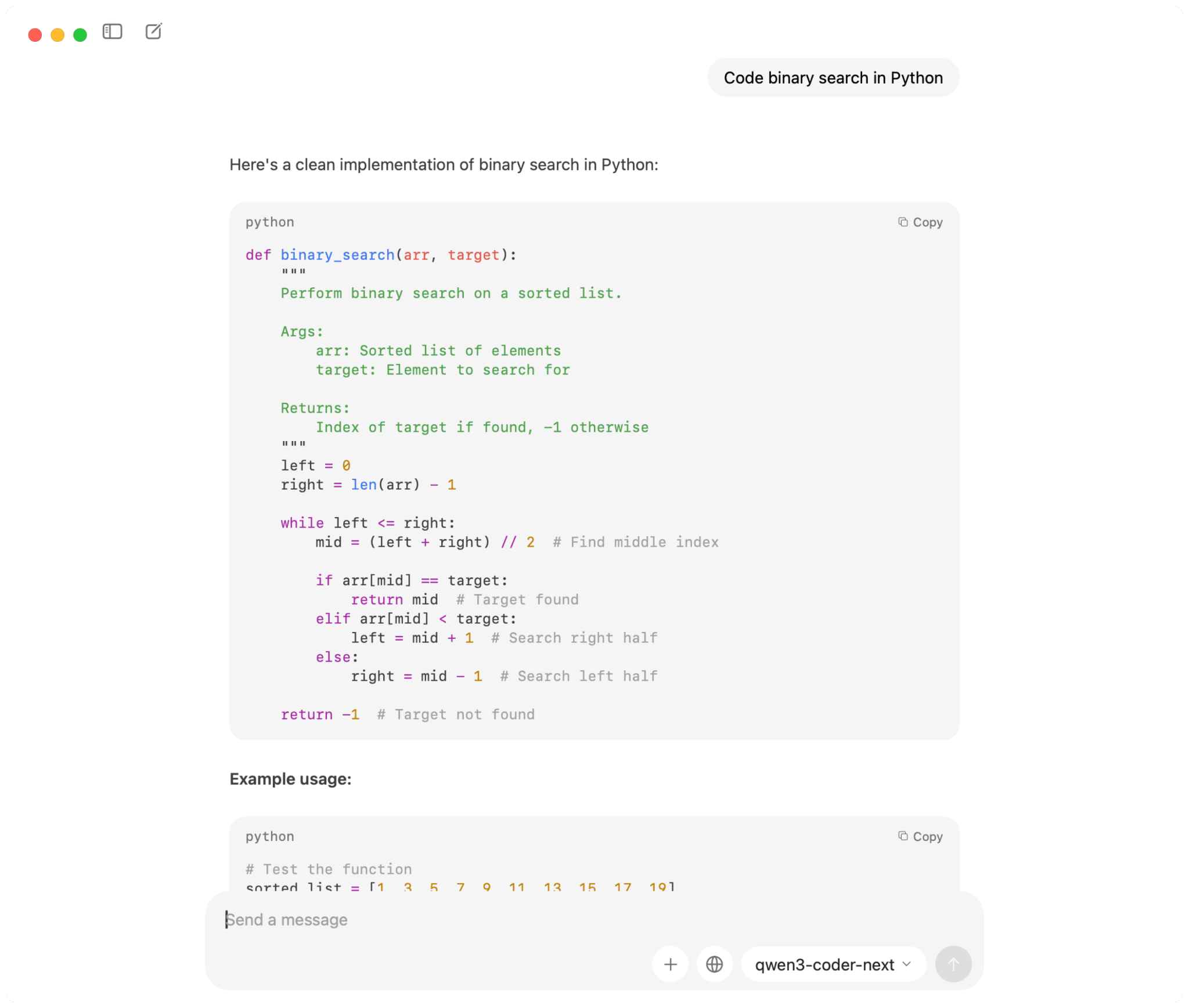
Using the ollama version of Qwen3-Coder-Next locally, the model takes about 48.2 GB of storage space and 51 GB of RAM.

Figure 15: Running Qwen3-Coder-Next locally.

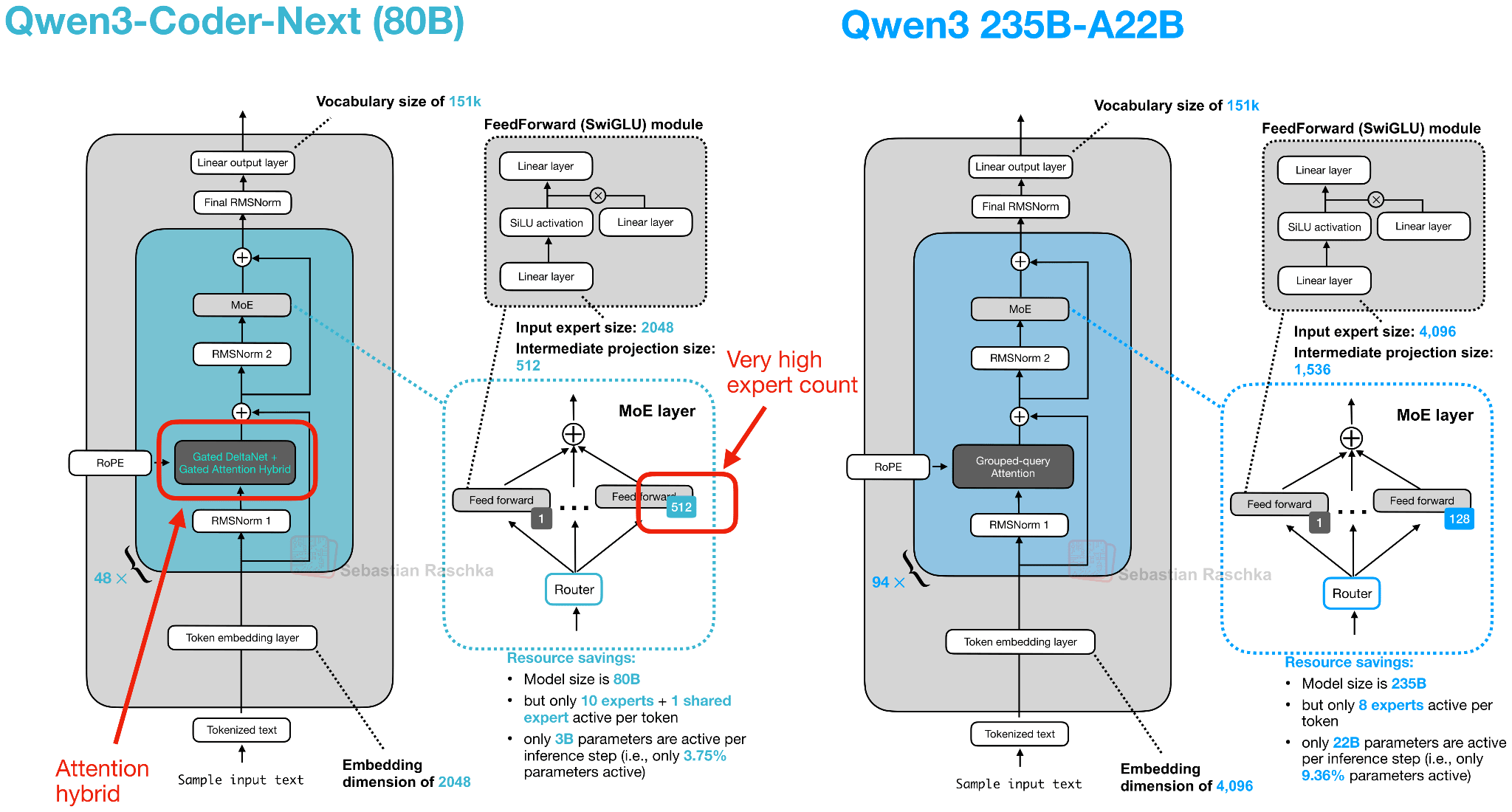
Note that the architecture behind Qwen3-Coder-Next is exactly the same as Qwen3-Next 80B (in fact, the pre-trained Qwen3-Next 80B is used as a base model for further mid- and post-training). Figure 16 below shows the Qwen3-Next architecture next to a regular Qwen3 235B model for reference.

Figure 16: Qwen3-Coder-Next 80B (3B parameters active per token) and the 3x larger Qwen3 235B-A22B architecture.

The new Qwen3 Next architecture stands out because, despite being 3x smaller than the previous 235B-A22B model, it introduces four times as many experts and even adds a shared expert. Both of these design choices (a high expert count and the inclusion of a shared expert).

​The other highlight is that they replace the regular attention mechanism with a Gated DeltaNet + Gated Attention hybrid, which helps enable the native 262k token context length in terms of memory usage (the 235B-A22B model supported 32k natively and 131k with YaRN scaling).

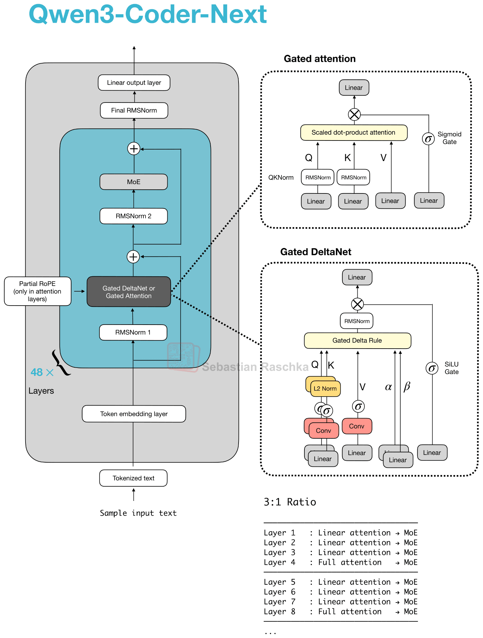
​So how does this new attention hybrid work? Compared to grouped‑query attention (GQA), which is still standard scaled dot‑product attention (sharing K/V across query‑head groups to cut KV‑cache size and memory bandwidth as discussed earlier, but whose decode cost and cache still grow with sequence length), their hybrid mechanism mixes Gated DeltaNet blocks with Gated Attention blocks in a 3:1 ratio as shown in Figure 17.

Figure 17: The Qwen3-Coder-Next attention hybrid setup.

We can think of the gated attention block as standard scaled-dot-product attention used in GQA, with a few tweaks on top. The main differences between gated attention and plain GQA block are:

  1. an output gate (sigmoid-controlled, usually per-channel) that scales the attention result before it is added back to the residual;

  2. zero-centered RMSNorm for QKNorm, rather than a standard RMSNorm;

  3. partial RoPE (on a subset of dimensions).

Note that these are essentially just stability changes to GQA.

The Gated DeltaNet is a more significant change. In the DeltaNet block, q, k, v, and two gates (α, β) are produced by linear and lightweight convolutional layers with normalization, and the layer replaces attention with a fast‑weight delta rule update.

However, the tradeoff is that DeltaNet offers less precise content‑based retrieval than full attention, which is why one gated attention layer remains.

Given that attention grows quadratically, the DeltaNet component was added to help with memory efficiency. In the “linear-time, cache-free” family, the DeltaNet block is essentially an alternative to Mamba. Mamba keeps a state with a learned state-space filter (essentially a dynamic convolution over time). DeltaNet keeps a tiny, fast-weight memory updated with α and β, and reads it with q, using small convolutions only to help form q, k, v, α, β.

For more details on the attention hybrid and Qwen3-Next architecture, please see my previous article Beyond Standard LLMs.

​Since this article is primarily focused on LLM architectures, the training details are outside its scope. However, interested readers can find more information in their detailed technical report on GitHub.

5. z.AI’s GLM-5: A New Flagship Open-Weight Model

The GLM-5 release on February 12th was a big deal, because at the time of its release it appeared to be on par with the major flagship LLM offerings, including GPT-5.2 extra-high, Gemini Pro 3, and Claude 4.6 Opus. (That said, benchmark performance does not necessarily translate to real-world performance.)

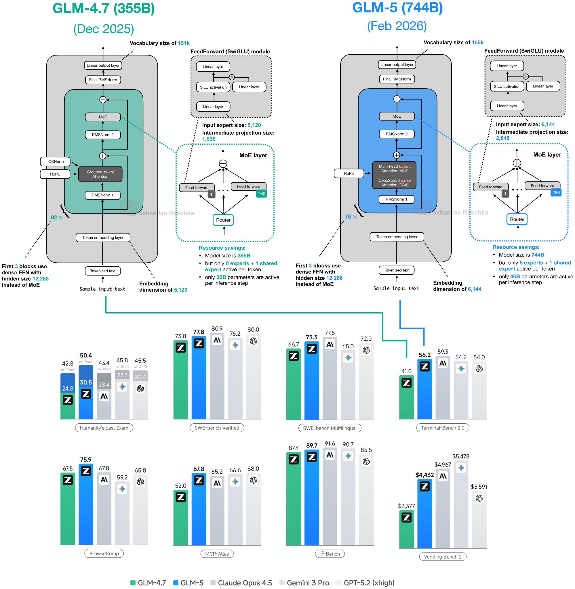
Figure 18: GLM-5 architecture next to its GLM-4.7 predecessor. Benchmarks at the bottom taken from the official GLM-5 technical report.

Not too long ago, GLM-4.7 (December 2025) was one of the strongest open-weight models. GLM-5 shows a major modeling performance improvement based on the benchmark shown in Figure 18 above. That jump is likely partly due to improvements to the training pipeline, but likely largely attributed to its 2x larger parameter count from 355B parameters in GLM-4.7 to 744B parameters in GLM-5. This size increase now places GLM-5 between DeepSeek V3.2 (671B) and Kimi K2.5 (1T) in terms of scale.

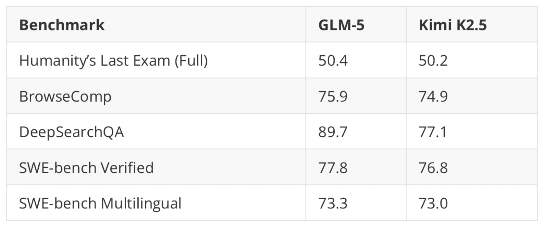
Comparing the benchmark numbers of the previously discussed Kimi K2.5 (1T), the smaller GLM-5 (744B) model seems slightly ahead, as shown in the table below.

Figure 19: GLM-5 (744B) and Kimi K2.5 (1T) benchmark performance side by side (larger is better).

Like GLM-4.7, all the other models discussed so far, GLM-5 is a Mixture-of-Experts model. The number of active parameters per token increases only slightly, from 32B in GLM-4.7 to 40B in GLM-5.

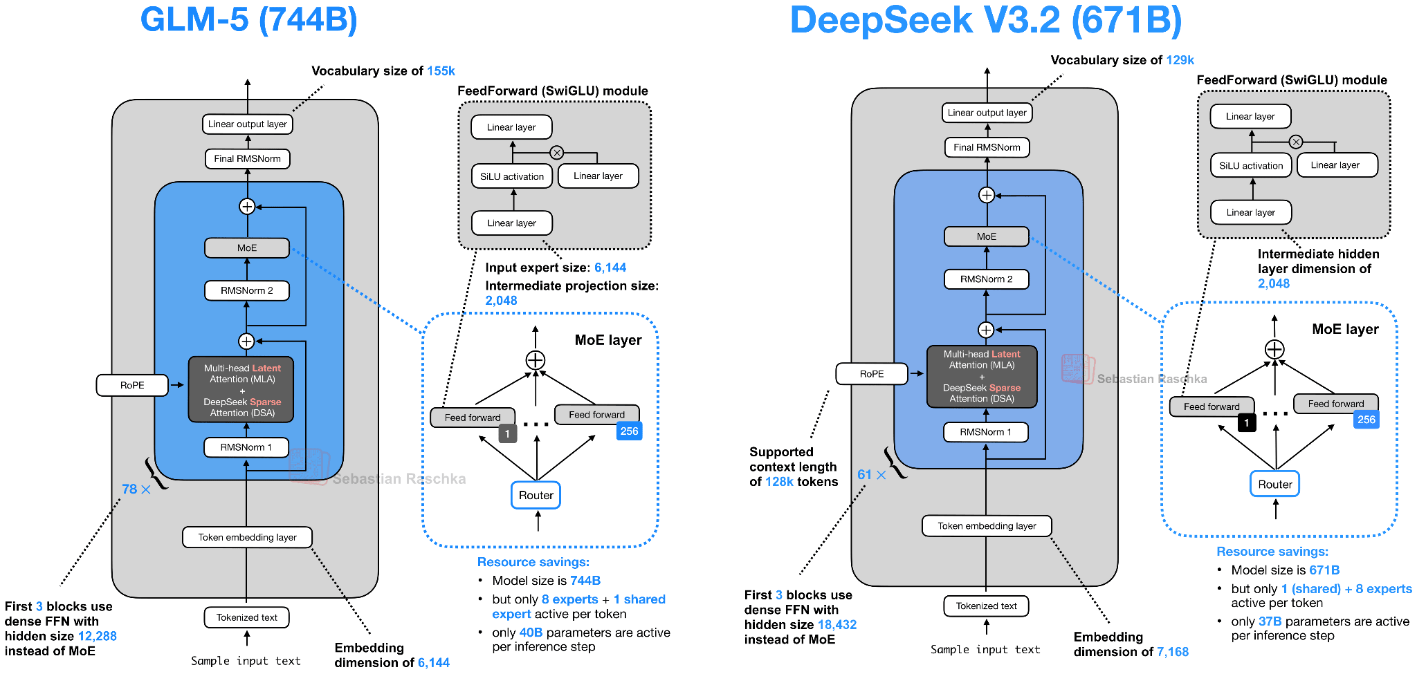
As shown in Figure 20 below, GLM-5 now adopts DeepSeek’s multi-head latent attention as well as DeepSeek Sparse Attention. (I described DeepSeek Sparse Attention in more detail in From DeepSeek V3 to V3.2: Architecture, Sparse Attention, and RL Updates.)

These modifications are likely intended to reduce inference costs when working with long contexts. Otherwise, the overall architecture remains relatively similar.

Figure 20: GLM-5 and DeepSeek V3.2 side by side (two similar architectures at a similar size).

The increase in total size over GLM-4.7 mainly comes from expanding the number of experts, from 160 (GLM-4.7) to 256 (GLM-5), and slightly increasing layer dimensions (while keeping the number of experts the same at 8 regular + 1 shared expert per token). For example, the embedding dimension and expert size increase from 5,120 to 6,144, and the intermediate projection size rises from 1,536 to 2,048.

Interestingly, the number of transformer layers is reduced from 92 in GLM-4.7 to 78 in GLM-5. I assume this change is also intended to reduce inference costs and improve latency, since layer depth cannot be parallelized in the same way as width.

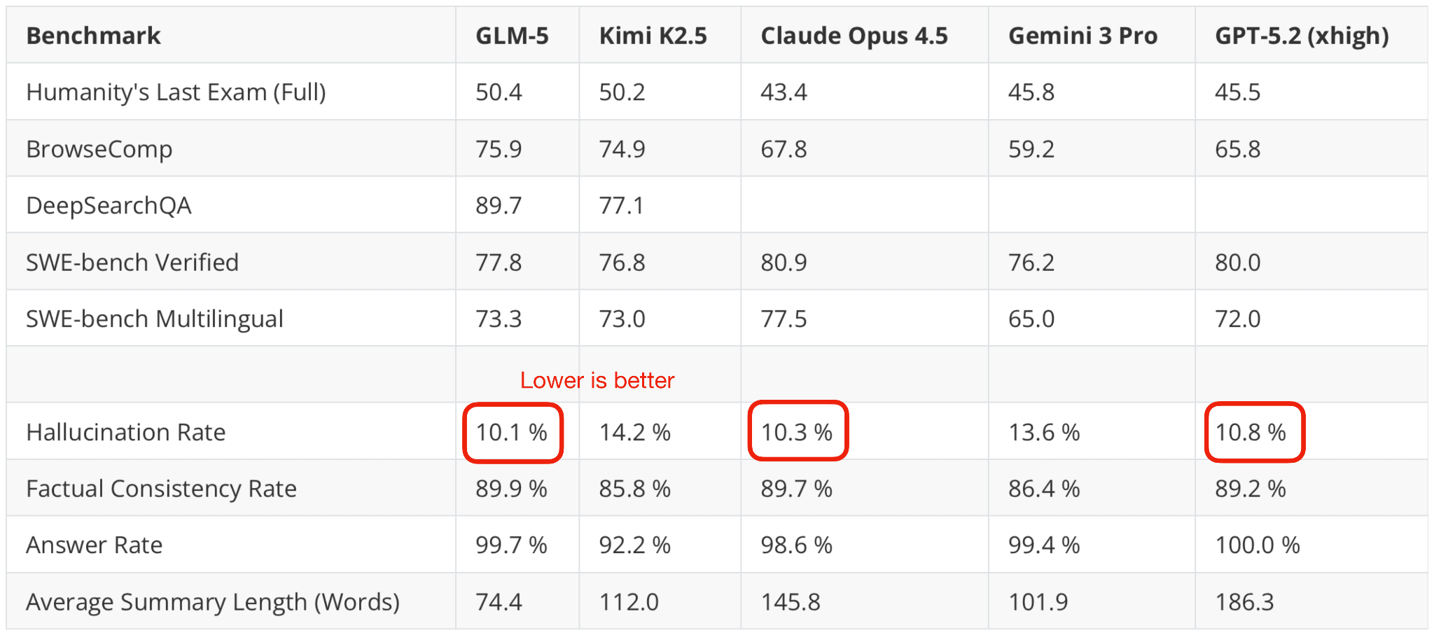
Additionally, I also checked an independent benchmark (here, the hallucination leaderboard), and it indeed looks like GLM-5 is on par with Opus 4.5 and GPT-5.2 (while using fewer tokens).

Figure 21: Next to the overall benchmark performance, this table adds hallucination rates from the hallucination leaderboard.

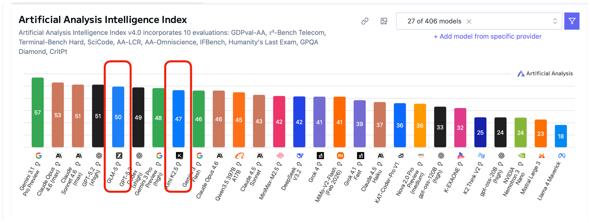
Furthermore, looking at the most recent Artificial Intelligence Index, which aggregates various benchmarks, GLM-5 is indeed slightly ahead of Kimi K2.5 and only one point behind GPT-5.2 (xhigh) and the recent Claude Sonnet 4.6.

Figure 22: Artificial Intelligence Index snapshot from Feb 21, 2026.

6. MiniMax M2.5: A Strong Coder with “Only” 230B Parameters

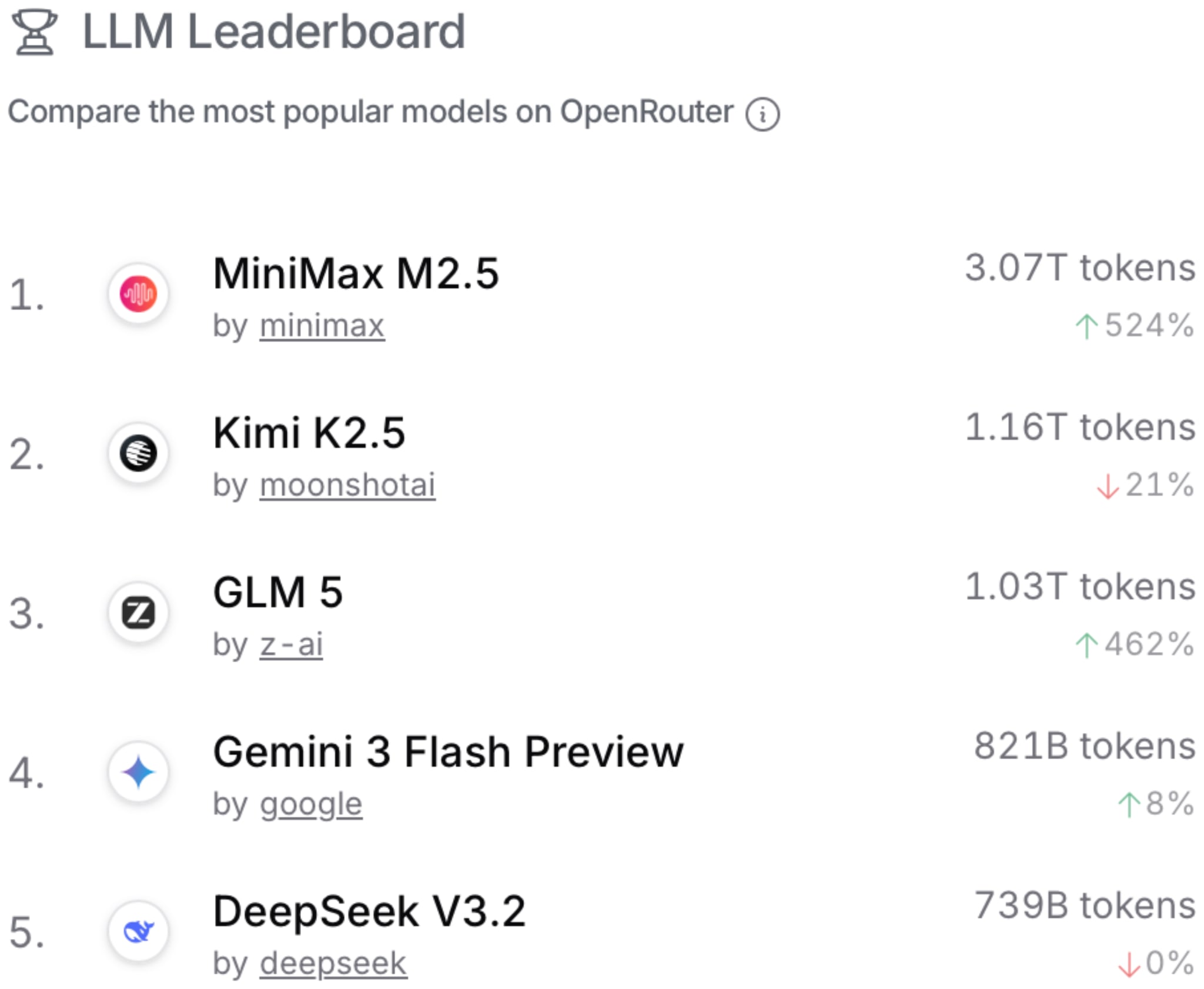
The aforementioned GLM-5 and Kimi K2.5 are popular open-weight models, but according to OpenRouter statistics, they pale in comparison to MiniMax M2.5, which was released on February 12 as well.

Figure 23: OpenRouter usage snapshot from Feb 21, 2026.

​

OpenRouter is a platform and API that lets developers access and route requests across many different LLMs from various providers. Note that while its usage statistics are a good indicator of open-weight model popularity, it’s heavily biased towards open-weight models (versus proprietary models), since most users use proprietary models through the official platform directly. There is also usage bias across open-weight models, since many people also use open-weight models through the official developers’ APIs. Anyways, it can still be an interesting place to guesstimate the relative popularity of open-weight models that are too large to run locally for most users.

​

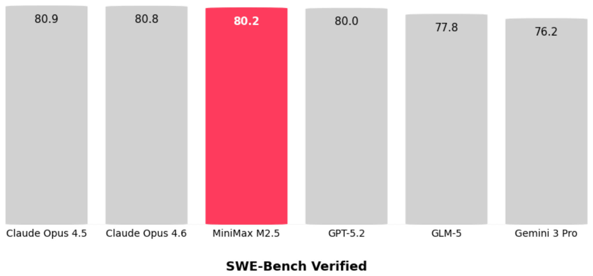
Now, back to MiniMax M2.5. Pulling together the GLM-5 data from the SWE-Bench Verified coding benchmark and combining it with the reported MiniMax M2.5, the latter appears to be a slightly stronger model (at least when it comes to coding).

Figure 24: MiniMax M2.5 coding performance on SWE-Bench Verified​

Side note: It’s interesting to see Opus 4.5 and Opus 4.6 practically scoring identically on SWE-Bench Verified. This can be an indicator that LLM progress has stalled. I don’t think that’s true, though, given that users of Opus 4.6 can confirm that this model does seem to perform better in real-world usage. So, the more likely issue here is that the SWE-Bench Verified benchmark has saturated, and it may no longer be a meaningful benchmark to report from now on (in favor of other benchmarks like SWE-Bench Pro, for example). With saturated, I mean that it potentially contains unsolvable problems due to design issues (as discussed in a recent Reddit thread and the new “Why SWE-bench Verified no longer measures frontier coding capabilities“ article by OpenAI).

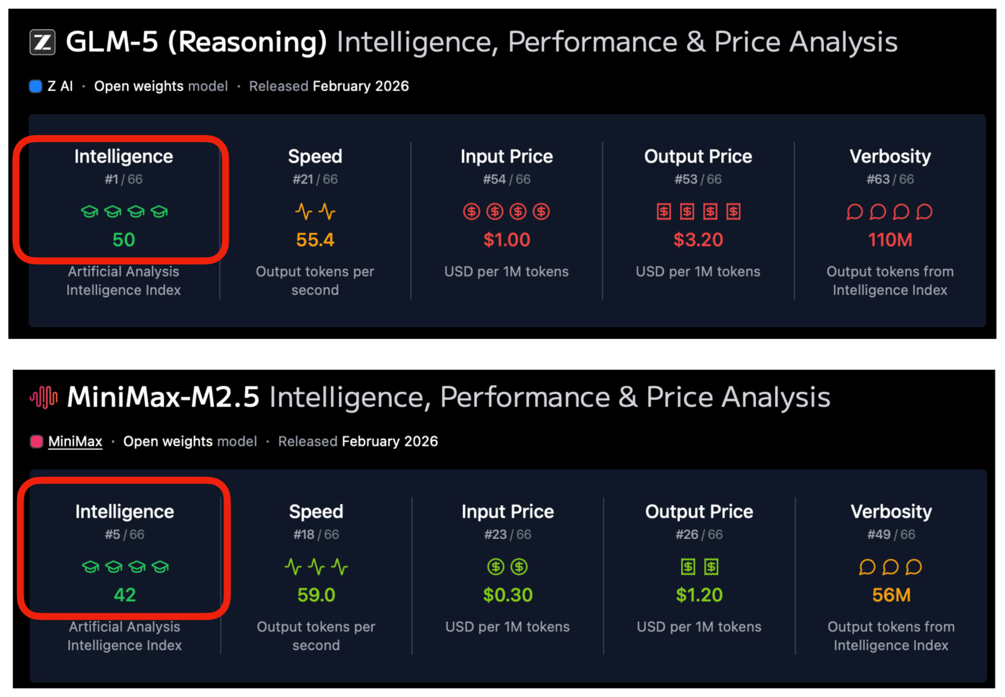
Anyways, back to the topic of MiniMax M2.5 performance. Looking across a broader selection of benchmarks, according to the Artificial Intelligence Index aggregation, GLM-5 remains ahead. This is perhaps no surprise because GLM-5 is still a 4x larger model than M2.5, even though the tokens/sec throughput is quite similar.

Figure 25: GLM-5 vs MiniMax M2.5 comparison based on the Artificial Intelligence Index (Feb 21, 2026)

I think MiniMax M2.5’s popularity is partly owed to the fact that it is a smaller, cheaper model with roughly similar modeling performance (i.e., a good bang for the buck).

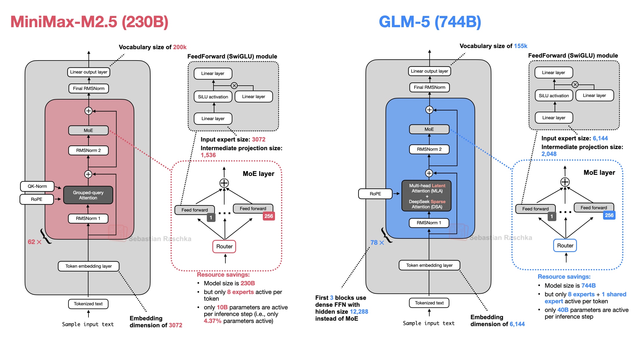
Architecture-wise, MiniMax M2.5 is a 230B model with a fairly classic design: just plain Grouped Query Attention, no sliding window attention or other efficiency improvements.

Figure 26: MiniMax M2.5 next to GLM-5.

So far, this is also the first architecture in this report that doesn’t come with a detailed technical report, but you can find additional information on the model hub page.

7. Nanbeige 4.1 3B: A Strong Llama 3 Successor

In this section, we are switching gears and finally covering a smaller model that can run locally on a laptop. But first let’s start with some context before we get to Nanbeige 4.1 3B.

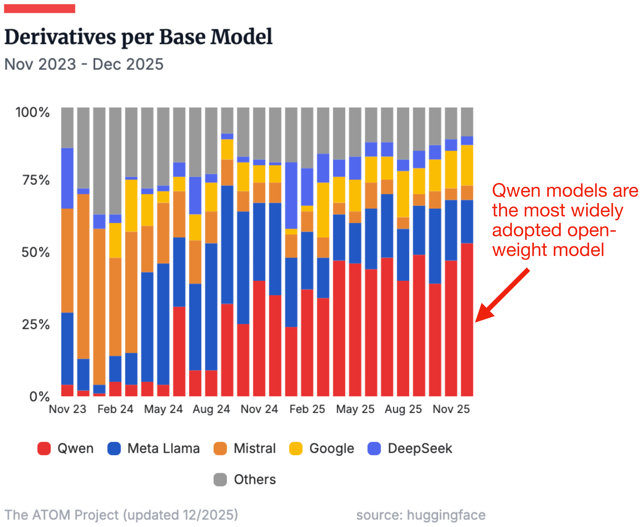
Qwen models have always been very popular models. I often tell the story that when I was an advisor during the NeurIPS LLM efficiency challenge a few years back, most of the winning solutions were based on a Qwen model.

​Now, Qwen3 is likely among the most widely used open-weight model suite since they cover such a wide range of sizes and use cases (from 0.6B to 235B)

Especially the smaller models (80B and less, like Qwen3-Next, covered previously) are great for local use on consumer hardware.

Figure 27: Relative adoption popularity of open-weight models. Note that this shows the number of models on the Hugging Face model hub that are finetuned using one of those models as a base model. (This is not the number of people who use the models on their computer locally, which would be a number impossible to know.) Source: Atom Project.​

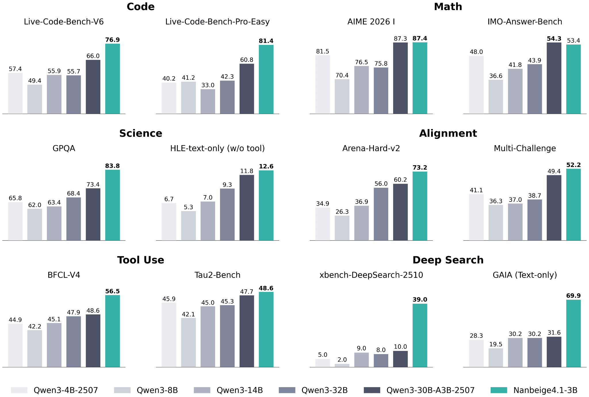
Why I am mentioning all this is that Nanbeige 4.1 3B seems to target the “small” LLM on-device use case that Qwen3 is so popular for. According to the Nanbeige 4.1 3B benchmarks, their model is way ahead of Qwen3 (perhaps no surprise, given that Qwen3 is almost a year old).

Figure 28: Nanbeige 4.1 3B benchmark comparison with Qwen3 (Source: Nanbeige 4.1 3B model hub page).

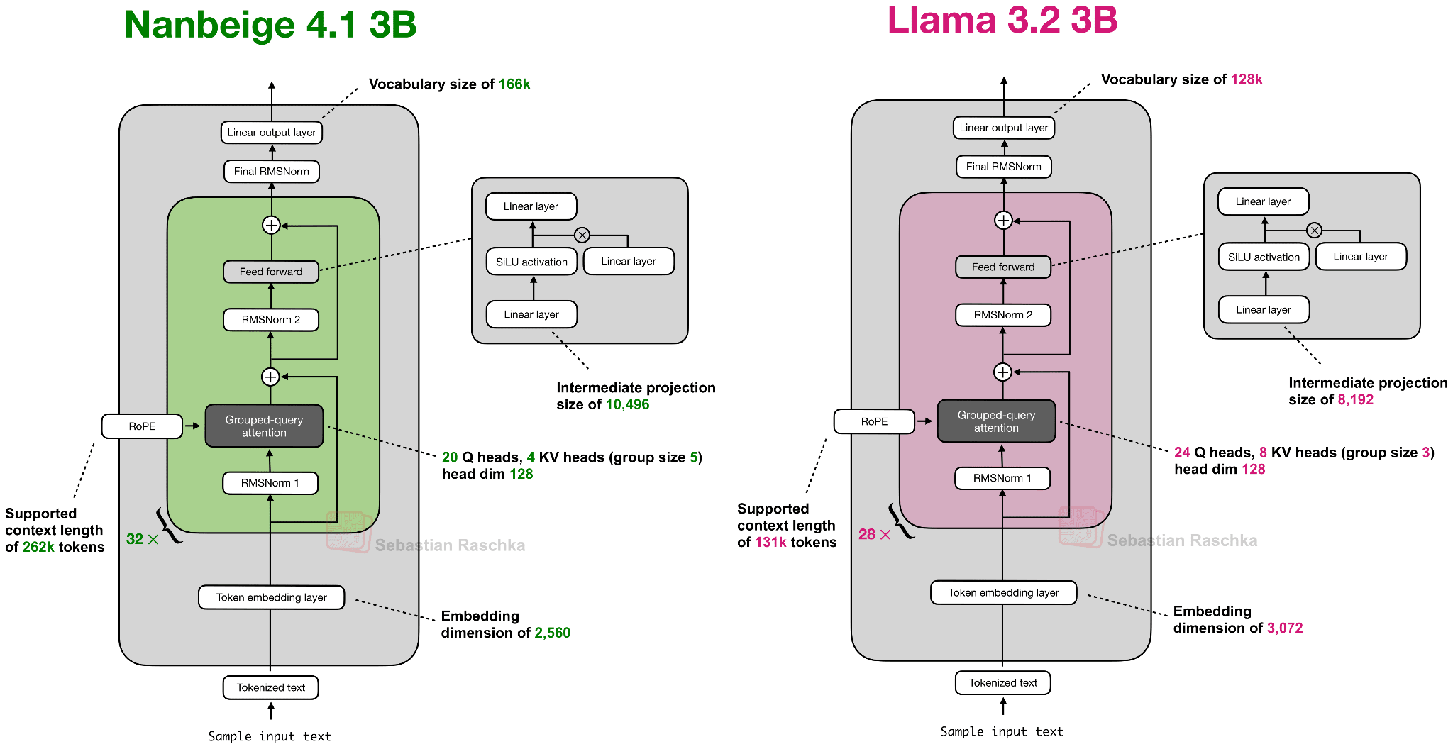
Architecture-wise, Nanbeige 4.1 3B is similar to Qwen3 4B, which is, in turn, very similar to Llama 3.2 3B. I am showing Nanbeige 4.1 3B next to Llama 3.2 3B below because it is the most similar in size.

Figure 29: Nanbeige 4.1 3B next to Llama 3.2 3B.

Nanbeige 4.1 3B uses the same architectural components as Llama 3.2 3B, with some minor scaling differences (slightly smaller embedding dimensions and larger intermediate projections, and so on). The one difference not shown in the figure above is that Nanbeige does not tie the input embedding weights to the output layer weights, whereas Llama 3.2 3B does. (In my experience, weight tying is a nice way to reduce the total number of parameters, but it almost always results in worse training performance as evidenced by higher training and validation losses.)

​As mentioned before, this article focuses primarily on the architecture comparisons. And in this case, most of the performance gains (compared to the Nanbeige 4 3B predecessor) come from additional post-training with supervised fine-tuning and reinforcement learning, but interested readers can find more information in the detailed technical report.

8. Qwen3.5 and the Continuation of Hybrid Attention

While the previous section briefly covered Qwen3 as the most open-weight model family, it is getting a bit long in the tooth as its release is almost a year ago (if we don’t count the Qwen3-Next variants geared towards efficiency). However, the Qwen team just released a new Qwen3.5 model variant on February 15.

Qwen3.5 397B-A17B, a Mixture-of-Experts (MoE) with 397B parameters (17B active per token), is a step up from the largest Qwen3 model, which is 235B parameters in size. (There is also the 1 trillion-parameter Qwen3-Max model, but it was never released as an open-weight model.)

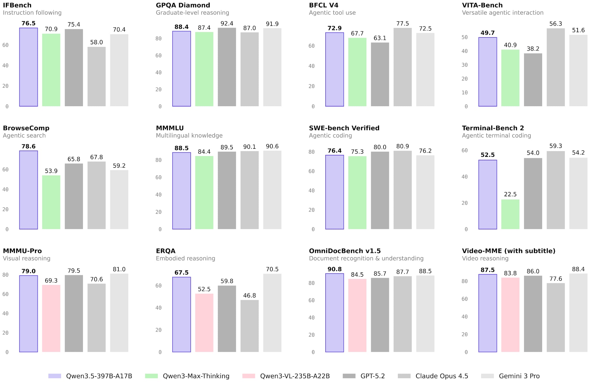
The obligatory benchmark overview shows that Qwen3.5 exceeds the previous Qwen3-Max model across the board, with a much stronger focus on agentic terminal coding applications (the main theme this year). Qwen3.5 appears to be roughly on par with GLM-5 and MiniMax M2.5 in terms of pure agentic coding performance (e.g., SWE-Bench Verified).​

Figure 30: Qwen3.5 benchmark overview from the official model hub page.

Since the Qwen team likes to release a separate coding model (e.g., see Qwen3-Coder-Next, which we discussed previously), this makes me curious to see how a potential Qwen3.5-Coder will perform.

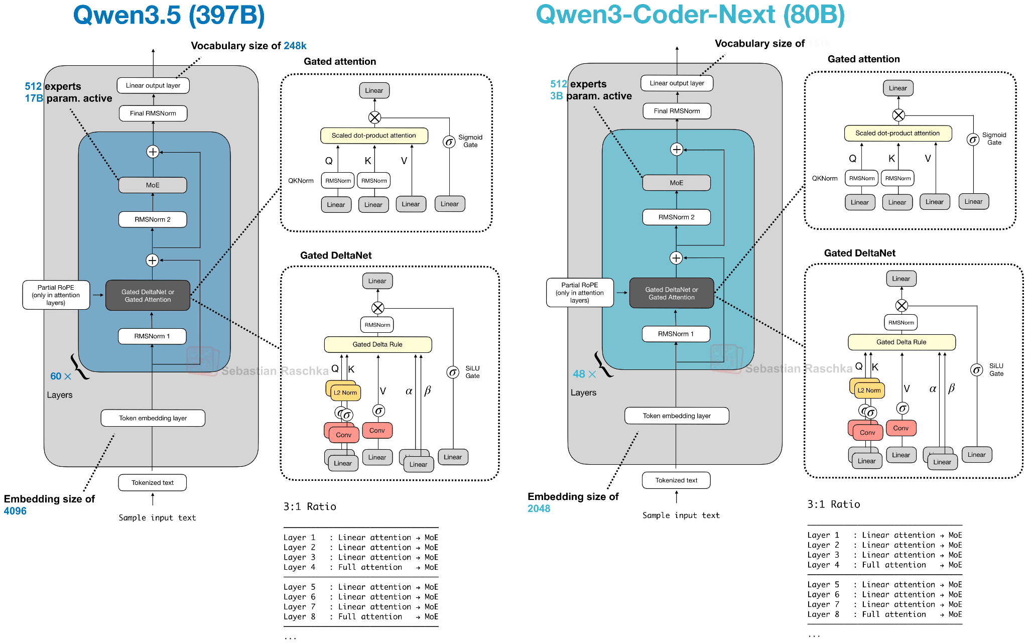
Architecture-wise, Qwen3.5 adopts the hybrid attention model (featuring Gated DeltaNet) that Qwen3-Next and Qwen3-Coder-Next (section 4) used. This is interesting because Qwen3-Next models were initially an alternative to the full-attention Qwen3 models, but this suggests that the Qwen team has now adopted the hybrid attention mechanism into its main line of models.

Figure 31: Comparison between Qwen3.5 and the Qwen3(-Coder)-Next architectures.​

Besides scaling up the model size, as shown in the figure above, Qwen3.5 now also includes multimodal support (previously, it was only available in separate Qwen3-VL models).

Anyways, Qwen3.5 is a nice refresh of the Qwen series, and I hope that we will see smaller Qwen3.5 variants in the future, too!

Edit: Just as I finalized this article, the Qwen team launched said smaller model variants:

9. Ant Group’s Ling 2.5 1T with Lightning Attention

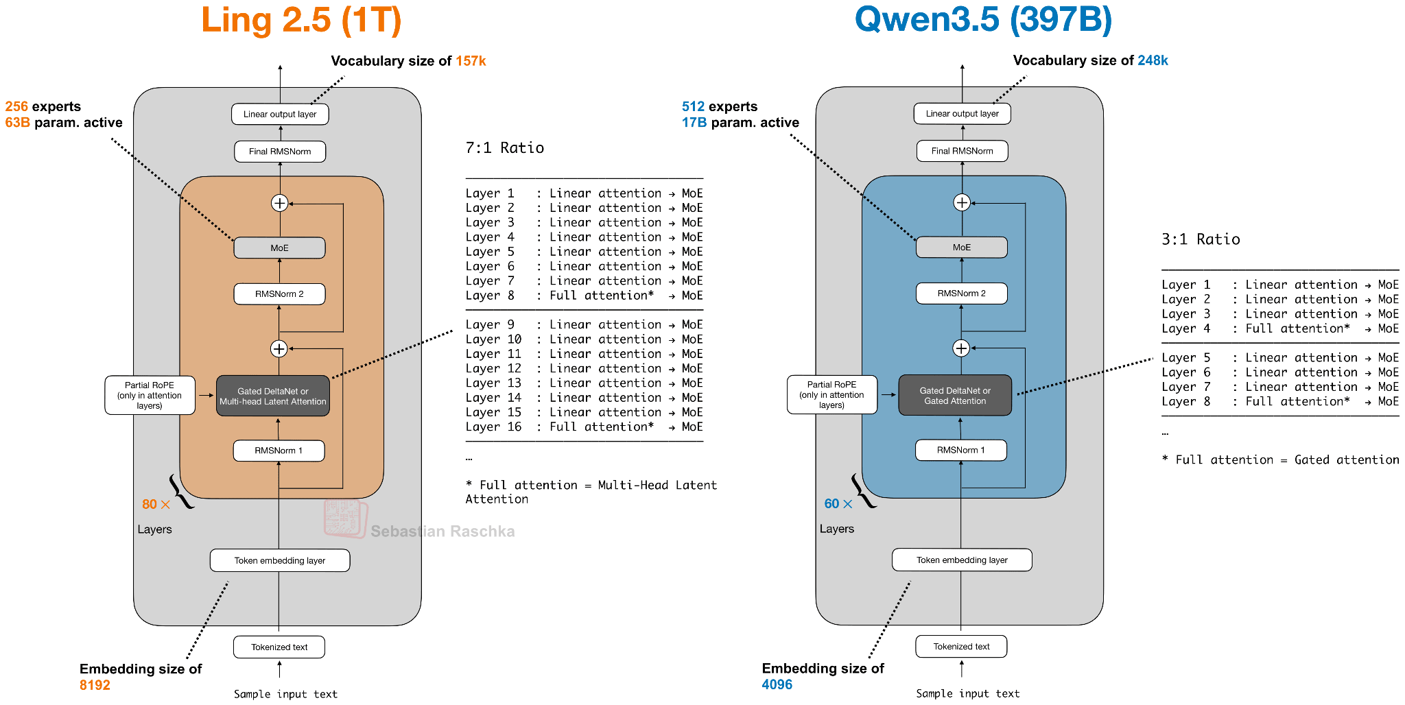
Ling 2.5 (and the reasoning variant Ring 2.5) are 1-trillion-parameter LLMs with a hybrid attention architecture in a similar spirit to Qwen3.5 and Qwen3-Next.

However, instead of Gated DeltaNet, they use a slightly simpler recurrent linear attention variant called Lightning Attention. In addition, Ling 2.5 adopts the Multi-Head Latent Attention (MLA) mechanism from DeepSeek.

Figure 32: Ling 2.5 compared to Qwen3.5; both architectures are linear attention hybrids.

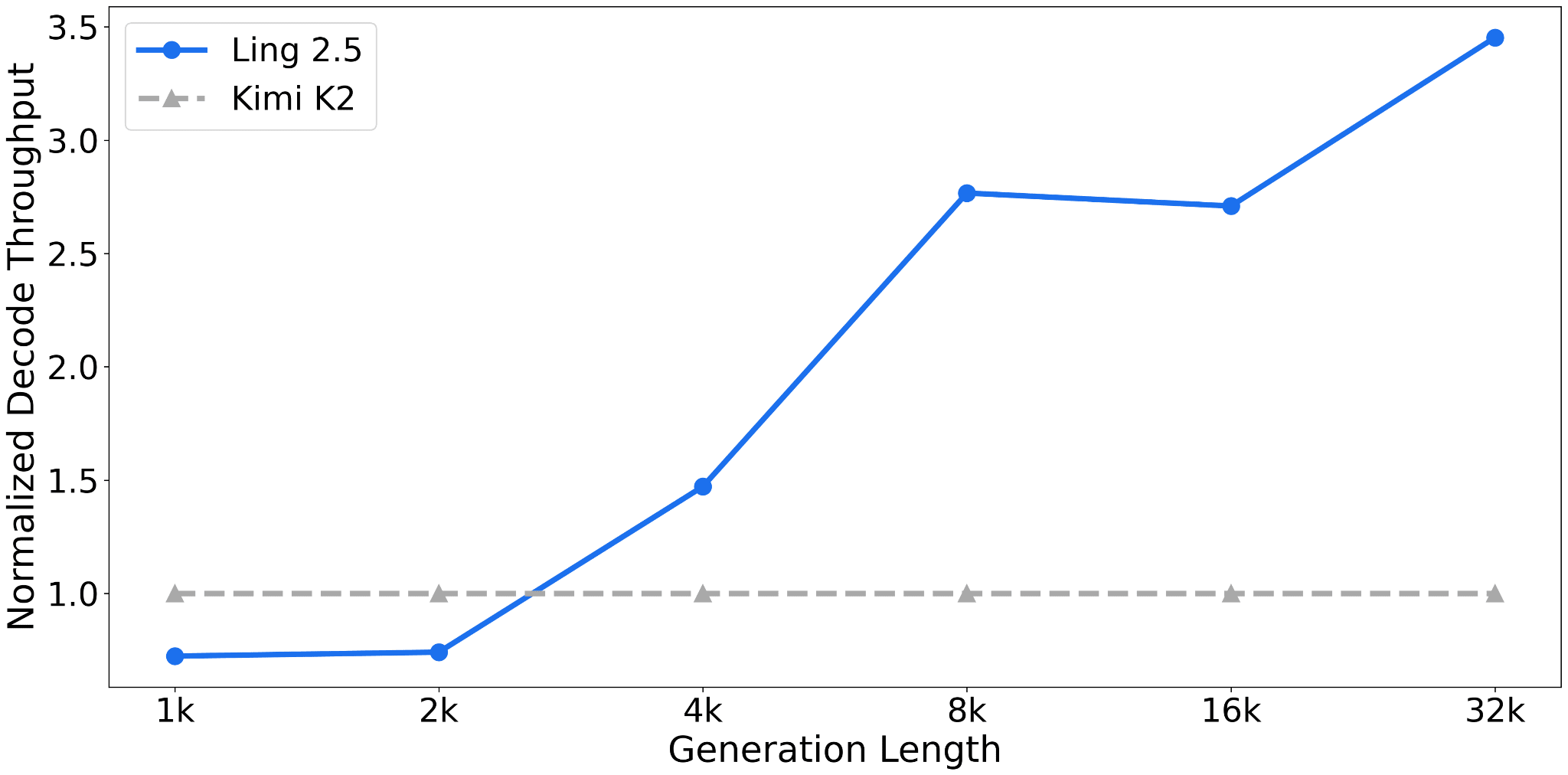
Ling 2.5 is not the strongest model in terms of absolute benchmark performance, but its selling point is very good efficiency in long contexts (due to the hybrid attention). Unfortunately, there are no direct comparisons to Qwen3.5, but compared to Kimi K2 (1T parameters; the same size as Ling 2.5), Ling 2.5 achieves a 3.5x higher throughput at a sequence length of 32k tokens.

Figure 33: Relative throughput of Ling 2.5 compared to Kimi K2 (same 1 trillion parameter size); note that the throughput is normalized so that Kimi K2 is shown at 1x (Kimi’s throughput is not linear even though it appears linear in this plot). Source: Ling 2.5 model hub page.

10. Tiny Aya: A 3.35B Model with Strong Multilingual Support

Released on February 17, Tiny Aya is a new, “small” LLM by Cohere that is said to be the “most capable multilingual open-weight model” at the 3B parameter size class. (Tiny Aya outperforms Qwen3-4B, Gemma 3 4B, and Ministral 3 3B according to the announcement post).

This is a great model to run and experiment with locally. The only caveat is that while it’s an open-weight model, its licensing terms are relatively restricted and only allow non-commercial use.

That aside, Aya is a 3.35B parameter model that comes in several flavors that are useful for

personal and (non-commercial) research use:

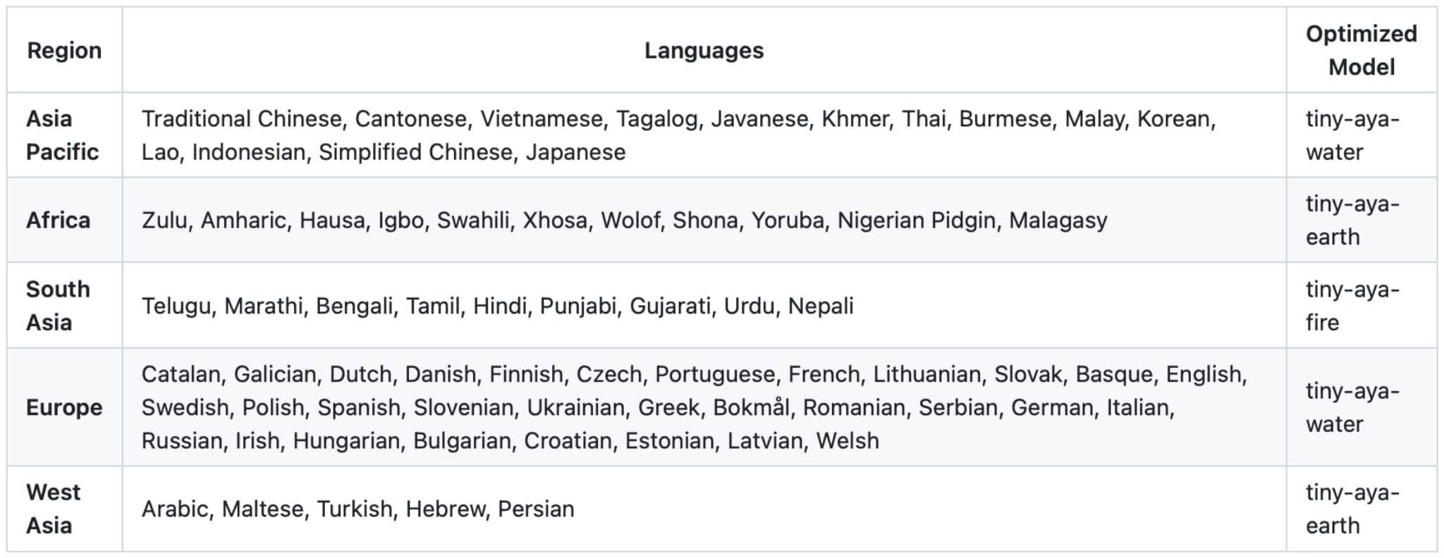
More specifically, below is a list of languages the models are optimized for.

Figure 34: Languages supported by the various Aya models.

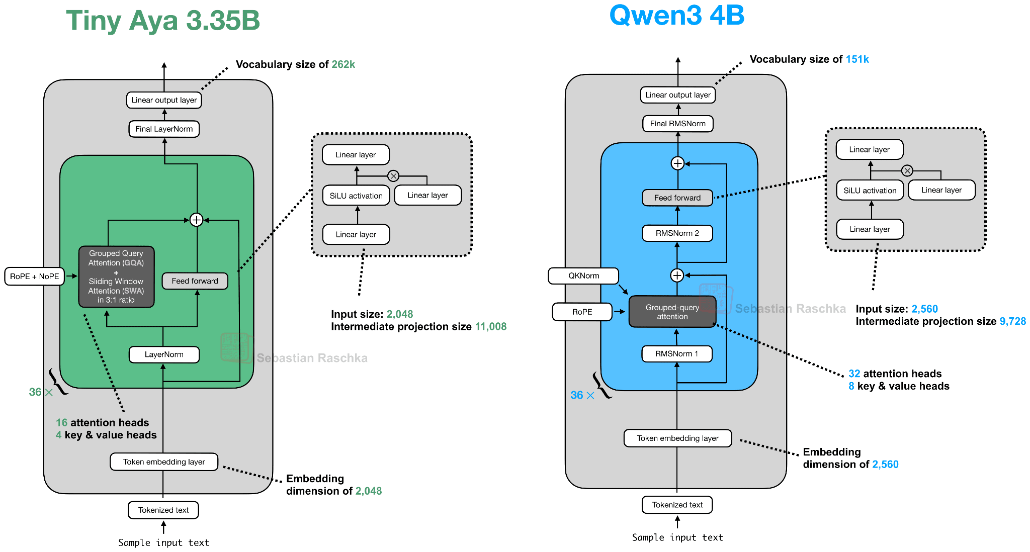
Architecture-wise, Tiny Aya is a classic decoder-style transformer with a few noteworthy modifications (besides the obvious ones like SwiGLU and Grouped Query Attention), as illustrated in the figure below.

Figure 35: Tiny Aya (featuring a parallel transformer block) and Qwen3 4B side by side.

Overall, the most noteworthy highlight in this architecture is the parallel transformer blocks. Here, the parallel transformer block computes attention and an MLP from the same normalized input, then adds both to the residual in a single step. I assume this is to reduce serial dependencies inside a layer to improve computational throughput.

For those readers familiar with Cohere’s Command-A architecture, Tiny Aya seems to be a smaller version of it. Also, an interesting detail is that the Tiny Aya team dropped QK-Norm (an RMSNorm applied to keys and queries inside the attention mechanism); QK-Norm has become quite standard for improving training stability in terms of reducing loss spikes. According to a developer on the Cohere team, QK-Norm was dropped “since it can interact with long context performance.”

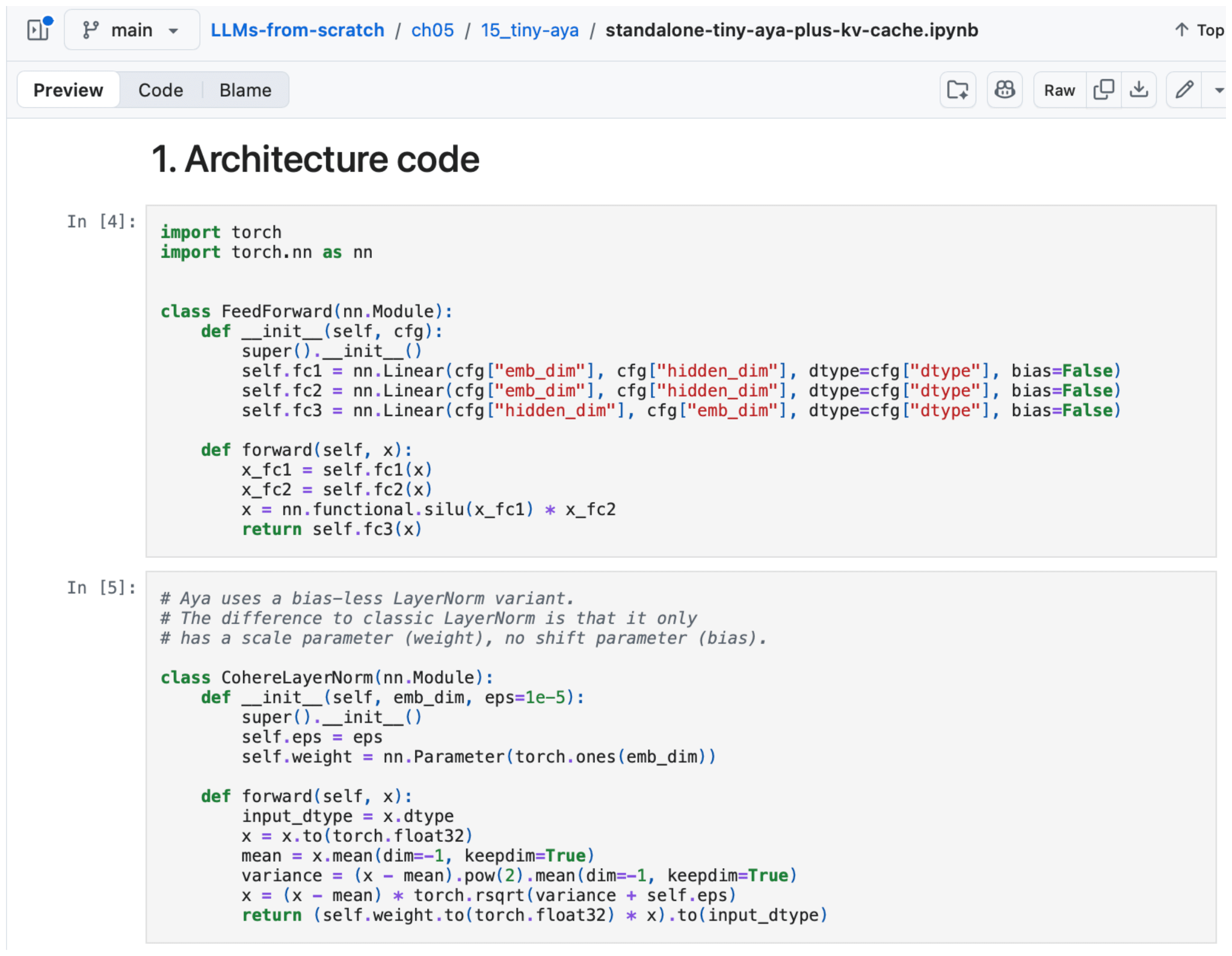
​As you may know, I occasionally code architectures from scratch. Since I found the parallel transformer block quite intriguing and the model runs fine on low-end hardware, I implemented it from scratch (for educational purposes), which you can find here on GitHub.

Conclusion

This article was quite the whirlwind tour covering the main open-weight LLM releases around February 2026. If there is a takeaway from this, it’s that there are various model architectures (all derived from the original GPT model) that work well. Modeling performance is likely not attributed to the architecture design itself but rather the dataset quality and training recipes (a good topic for a separate article).

​

That said, architectural design remains an essential part of building a successful LLM, and many developers seem to be steering towards adding more and more computational performance tweaks. For example, this includes adapting MLA (Kimi K2.5, GLM-5, Ling 2.5) and DeepSeek Sparse Attention (GLM-5) to continue the Gated DeltaNet (Qwen3.5) or similar forms of linear attention (Ling 2.5).

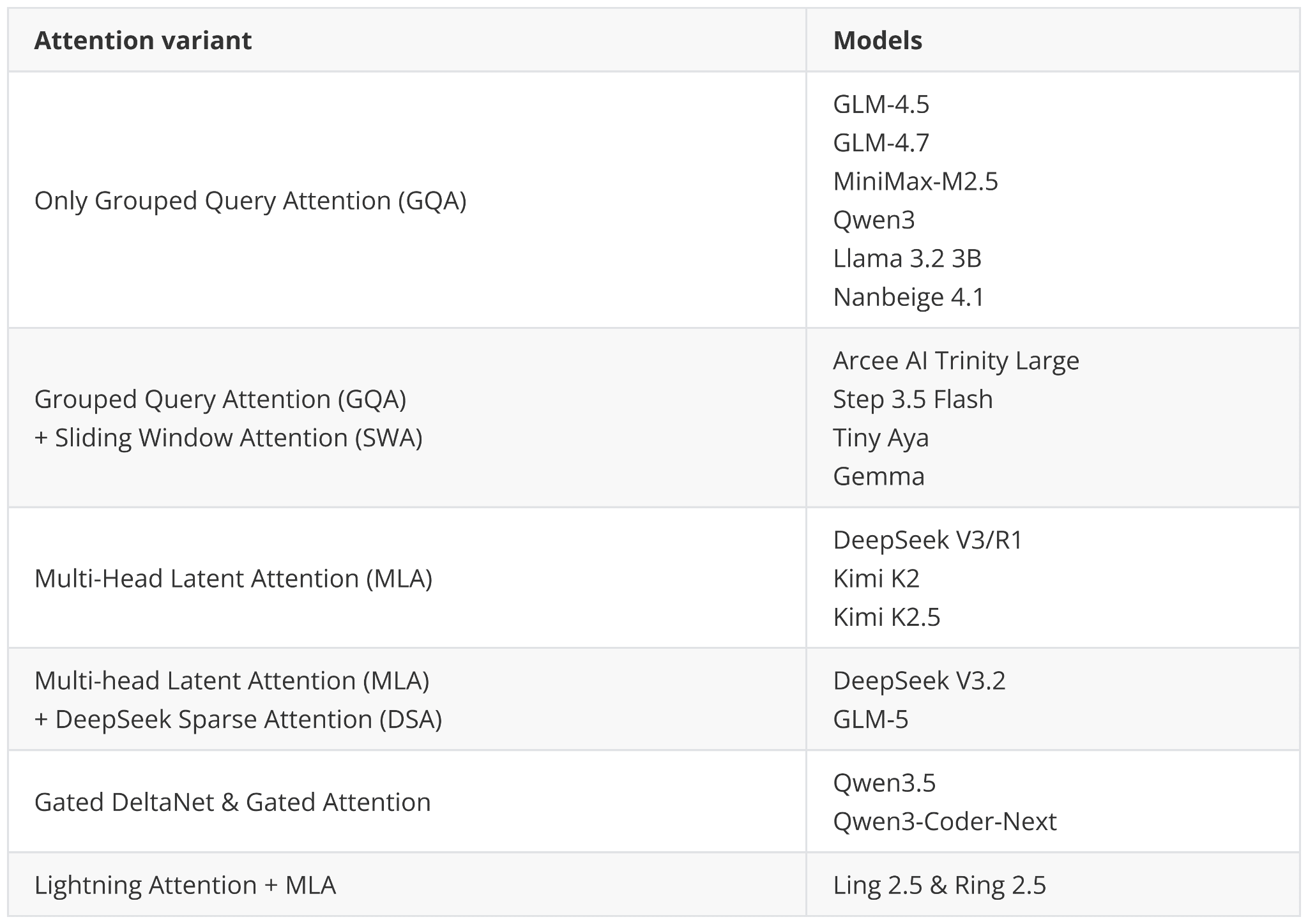
Figure 37: Attention types used by the various architectures mentioned in this article.

Also, more classic efficiency tweaks like grouped query attention and sliding window attention (Arcee Trinity, Step 3.5 Flash, Tiny Aya) remain popular. Among the new releases, only MiniMax M2.5 and Nanbeige 4.1 stayed very classic here, using only Grouped Query Attention without any other efficiency tweak.

DeepSeek V4

DeepSeek V4 is the model everyone is waiting for. Unfortunately, as of this writing, it hasn’t been released yet. However, I plan to add it to this article once it’s released, which is likely on or before the first week of March.

Another interesting model is Sarvam (30B & 100B) from India. The model was recently announced, but it hasn’t been released yet. Stay tuned for an update here as well.

Update 1: Sarvam 30B and 105B (Mar 6, 2026)

As promised, here is a short update on Sarvam.

While waiting for DeepSeek V4 we got two very strong open-weight LLMs from India.

There are two size flavors, Sarvam 30B and Sarvam 105B model (both reasoning models), which were released as open-weight models on March 6th alongside a fairly detailed announcement blog.

Interestingly, the smaller 30B model uses “classic” Grouped Query Attention (GQA), whereas the larger 105B variant switched to DeepSeek-style Multi-Head Latent Attention (MLA).

Figure 37: The Sarvam 30B and 105B architectures

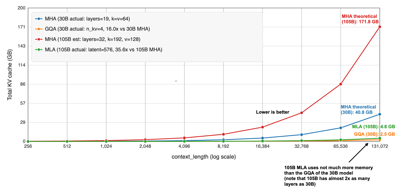
As I wrote about in my analyses before, both are popular attention variants to reduce KV cache size (the longer the context, the more you save compared to regular attention).

Figure 38: Relative efficiencies of GQA and MLA compared to MHA.

MLA is more complicated to implement, but it can give you better modeling performance if we go by the ablation studies in the 2024 DeepSeek V2 paper (as far as I know, this is still the most recent apples-to-apples comparison).

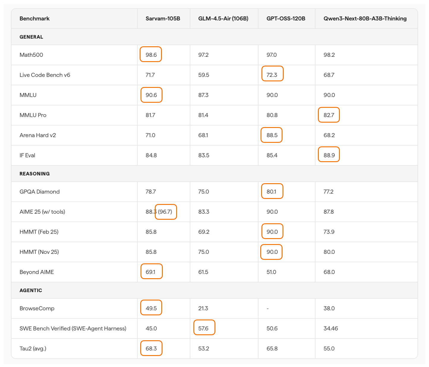
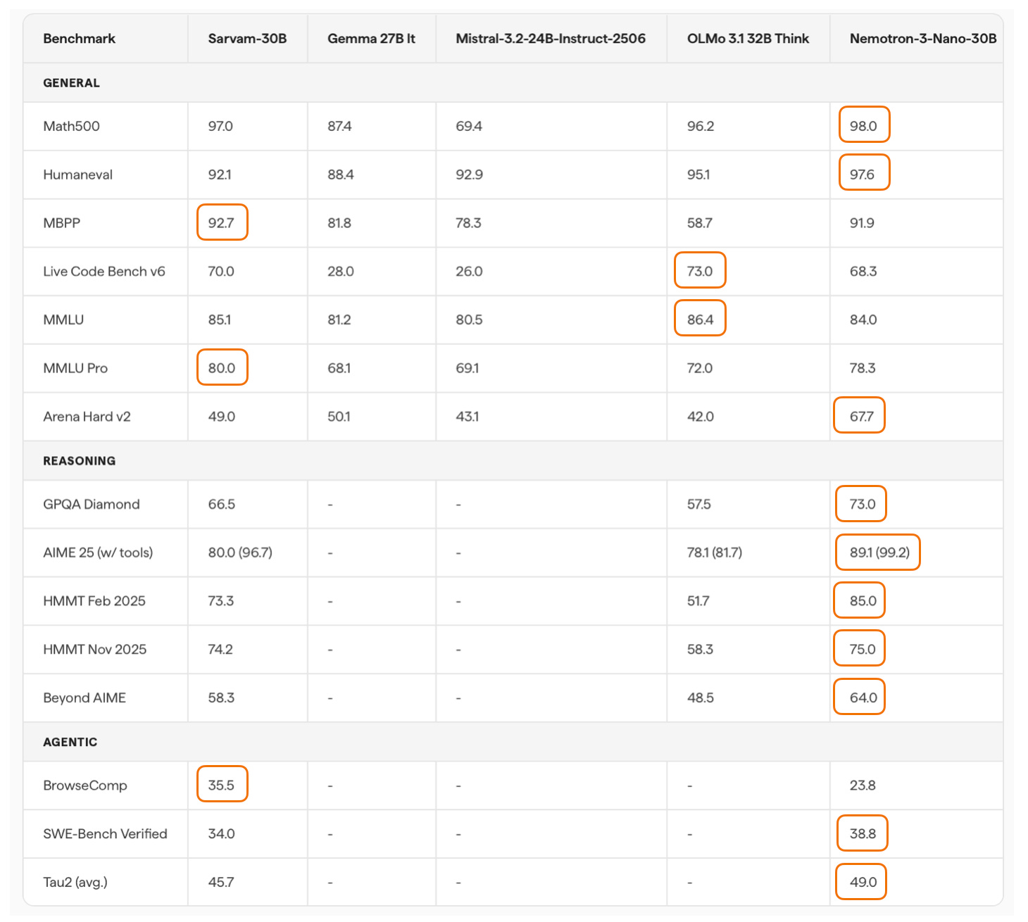
Speaking of modeling performance, the 105B model is on par with LLMs of similar size: gpt-oss 120B and Qwen3-Next (80B). Sarvam is better on some tasks and worse on others, but roughly the same on average.

Figure 39: Annotated benchmark (105B model) from the Sarvam blog post, with the best model in each row highlighted.

It’s not the strongest coder in SWE-Bench Verified terms, but it is surprisingly good at agentic reasoning and task completion (Tau2). It’s even better than Deepseek R1 0528 (not shown in the figure above).

Considering the smaller Sarvam 30B, the perhaps most comparable model to the 30B model is Nemotron 3 Nano 30B, which is slightly ahead in coding per SWE-Bench Verified and agentic reasoning (Tau2) but slightly worse in some other aspects (Live Code Bench v6, BrowseComp).

Figure 39: Annotated benchmark (30B model) from the Sarvam blog post, with the best model in each row highlighted.

Unfortunately, Qwen3-30B-A3B is missing in the benchmarks above, which is, as far as I know, is the most popular model of that size class. Interestingly, though, the Sarvam team compared their 30B model to Qwen3-30B-A3B on a computational performance analysis, where they found that Sarvam gets 20-40% more tokens/sec throughput compared to Qwen3 due to code and kernel optimizations.

One thing that is not captured by the benchmarks above is Sarvam’s good performance on Indian languages. According to a judge model, the Sarvam team found that their model is preferred 90% of the time compared to others when it comes to Indian texts. (Since they built and trained the tokenizer from scratch as well, Sarvam also comes with a 4 times higher token efficiency on Indian languages.


This magazine is a personal passion project, and your support helps keep it alive.

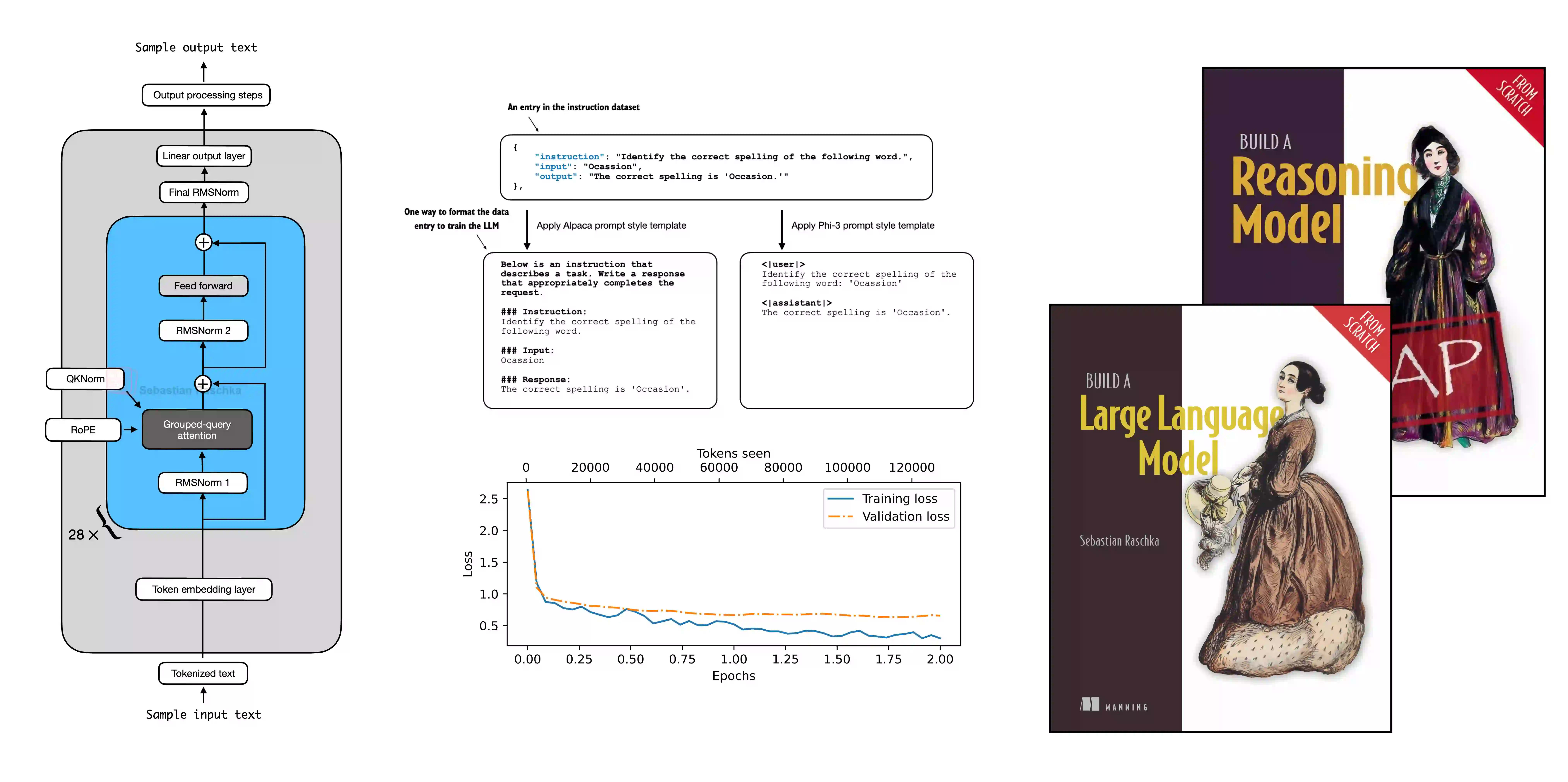
If you’d like to support my work, please consider a subscription or purchasing a copy of my Build a Large Language Model (From Scratch) book or its follow-up, Build a Reasoning Model (From Scratch). (I’m confident you’ll get a lot out of these; they explain how LLMs work in depth you won’t find elsewhere.)

Thanks for reading, and for helping support independent research!

Build a Large Language Model (From Scratch)
Build a Large Language Model (From Scratch) is now available on Amazon. Build a Reasoning Model (From Scratch) is in Early Access at Manning.

If you read the book and have a few minutes to spare, I’d really appreciate a brief review. It helps us authors a lot!

Your support means a great deal! Thank you!

❌