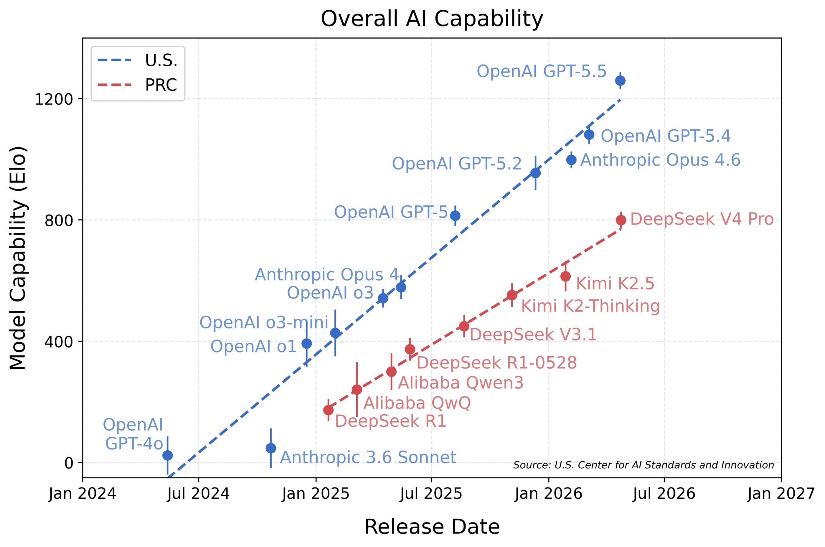
This month was packed, with all open frontier labs, including DeepSeek, releasing new models. The latter prompted an evaluation by the Center for AI Standards and Innovation (CAISI), which has evaluated open models and their risks in the past. Their result is that open models lag behind the American frontier, with the gap becoming wider over time:
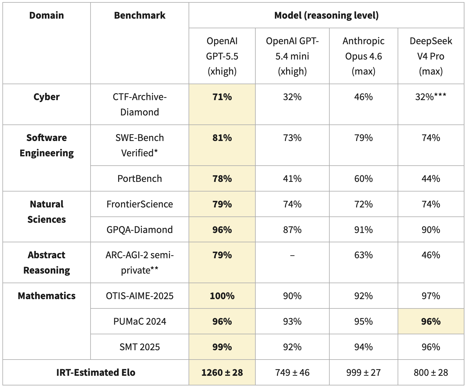
For the report, they calculate an Elo score based on Item Response Theory, which is commonly used to compare different models, even when they were tested on a different set of benchmarks. For V4, CAISI used nine different benchmarks:
The huge Elo difference is explained by DeepSeek V4s bad score in CTF-Archive-Diamond (which was only run with a subset of the benchmark and extrapolated with IRT for V4), PortBench (a CAISI-private benchmark) and ARC-AGI-2 (with a different scoring method than the public leaderboards). The differences in these benchmark have a huge impact on the overall Elo, which can exacerbate the difference in capabilities.
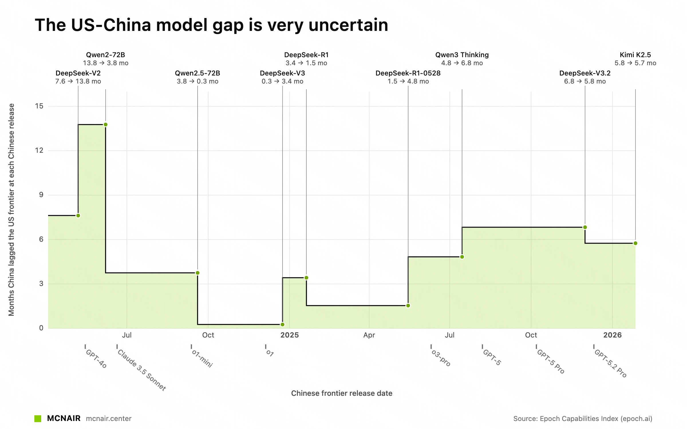
When using Epoch AI’s ECI, which also uses IRT over a set of different benchmarks, we see that the gap roughly stays between 3-7 months since R1:
The open<>closed gap in ECI (from https://mcnair.center/china/)
However, both CAISI and ECI paint an incomplete picture, as both use standardized (and simple) setups to compare the capabilities of models. To be more concrete: Coding tasks are evaluated using access to bash and a for-loop with a fixed budget of tokens, not with a harness such as Claude Code or OpenCode, which models are trained in! These setups result in benchmarks claiming that porting applications to another language is currently not possible, while Bun has been ported from Zig to Rust with 1 million LOC changes1.
Therefore, we would argue that a frontier comparison of open and closed models would also need to elicit the capabilities of all models better, which means the usage of the preferred harnesses, as well as model-specific prompting.
This section was written primarily by Florian. An interesting dynamic within Interconnects is that Florian believes more in the proximity of open frontier models to closed alternatives in true performance. Nathan thinks the benchmarks are imperfect as well, but thinks the closed models are ahead by more. We’re going to continue to unpack this in our future content.
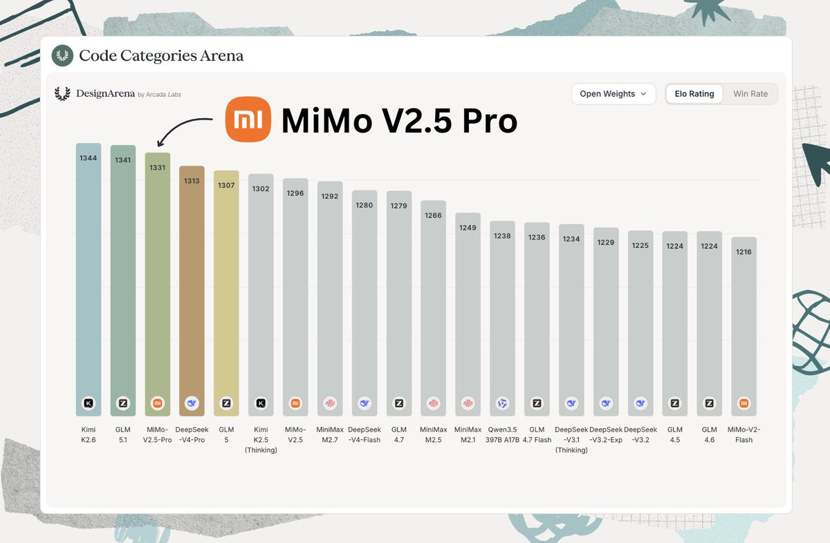
MiMo-V2.5-Pro by XiaomiMiMo: Avid Artifacts readers know that Xiaomi has been working on open models for a while; its debut was exactly one year ago. The progress of its releases is remarkable, with 2.5 Pro (released under Apache 2.0) being neck and neck with other flagship models such as Kimi K2.6 and GLM-5.1 in both benchmarks and real-world usage.
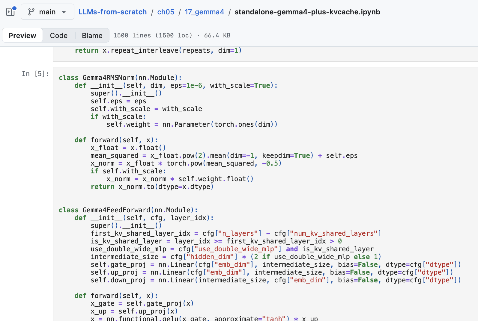
gemma-4-26B-A4B-it by google (full Interconnects post here): The long-awaited update to the Gemma series, featuring multiple sizes: 4B, 9B, and 31B dense models, as well as a 26B-A4B MoE. Even more importantly, with Gemma 4, Google has decided to use Apache 2.0 as its license, which removes the uncertainty and legal challenges around interpreting custom licenses.
Kimi-K2.6 by moonshotai: An update to the Kimi series, delivering stronger performance across the board and making it one of the best open models out there yet again. They also focus on long-horizon performance, showing that open models are capable of running over hours to complete tasks or optimize performance. Given the focus of everyone to build autoresearch-like systems, seeing open models catch up is important.
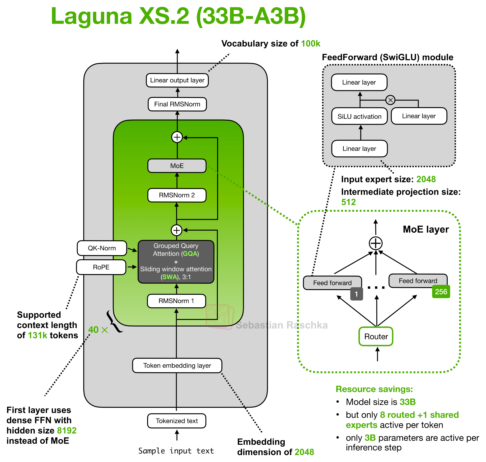
Laguna-XS.2 by poolside: Poolside AI has released its first public coding-focused models, including the open-weight XS.2. Its size (33B-A3B) makes it attractive for local use, with performance on par with other models in that size range. The accompanying blog post is worth a read, as is the deep dive into reward hacking during coding evaluations.
DeepSeek-V4-Flash by deepseek-ai: DeepSeek has finally released its successor to the V3 series, which it kept updating for months. It comes in two sizes: Pro, which is a 1.6T-A49B MoE, and Flash, a 284B-13B model. Based on others’ experience, the latter model seems to be the real star of the show, as its performance is relatively strong, while Pro seems to underdeliver relative to its size. The tech report goes into great detail, including the architectural changes used to achieve better and cheaper long-context performance.
Models
General Purpose
Qwen3.6-35B-A3B by Qwen: An update to the Qwen 3.5 series targeting one of the most widely used sizes.
LFM2.5-350M by LiquidAI: With 28T tokens for 350M parameters, this model might be the most overtrained model out there.
Trinity-Large-Thinking by arcee-ai: The reasoning version of Trinity, one of the best Western open models. It has topped the OpenRouter charts for a while and can power agentic applications such as OpenClaw.
GLM-5.1 by zai-org: An update to GLM-5, improving scores across the board. The focus for this update is on long-horizon tasks.
After a short family break, I am excited to be back and catching up on a busy few weeks of open-weight LLM releases. The thing that stood out to me is how much newer architectures are focused on long-context efficiency.
As reasoning models and agent workflows keep more tokens around (for longer), KV-cache size, memory traffic, and attention cost quickly become the main constraints, and LLM developers are adding a growing number of architecture tricks to reduce those costs.
The main examples I want to look at are KV sharing and per-layer embeddings in Gemma 4, layer-wise attention budgeting in Laguna XS.2, compressed convolutional attention in ZAYA1-8B, and mHC plus compressed attention in DeepSeek V4.
Most of these changes look like small tweaks in my architecture diagrams, but some of them are quite intricate design changes that are worth a more detailed discussion.
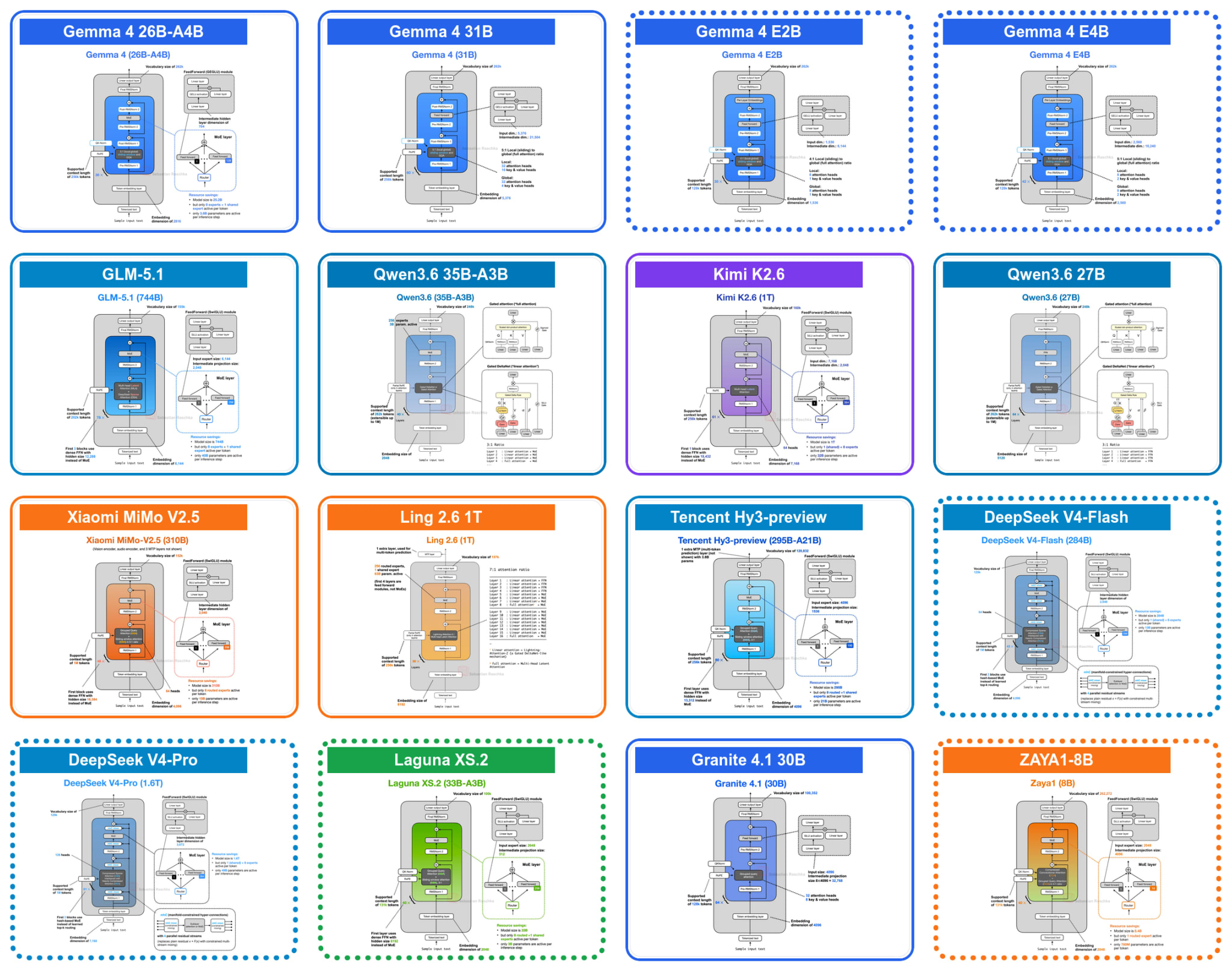
Figure 1. LLM architecture drawings of recent, major open-weight releases (April to May). You can find the images, and more details, in my LLM architecture gallery. Not all model sizes are shown; Qwen3.6 includes the 27B and 35B-A3B variants, and ZAYA1 is represented by the 8B model (omitting ZAYA1-base and ZAYA1-reasoning-base). The architectures in the dotted boxes are covered in more detail in this article.
Note that this article is about architecture designs, so I will mostly skip dataset mixtures, training schedules, post-training details, RL recipes, benchmark tables, and product comparisons. Even with that narrower scope, there is a lot to cover. And, like always, the article turned out longer than I expected, so I will keep the focus on what changes inside the transformer block, residual stream, KV cache, or attention computation.
Please also note that I am only covering those topics that are interesting (new) design choices and that I haven’t covered elsewhere, yet. This list includes:
KV sharing and per-layer embeddings in Gemma 4
Compressed convolutional attention in ZAYA1
Attention budgeting in Laguna XS.2
mHC and compressed attention in DeepSeek V4
Previous Topics
Before getting into the new parts, here are the two previous articles I will refer back to. The first one gives a broader architecture background on recent MoE models, routed experts, active parameters, and model-size comparisons. The second one covers the attention background that comes up repeatedly below, including MHA, MQA, GQA, MLA, sliding-window attention, sparse attention, and hybrid attention designs.
I also turned several of these explanations into short, standalone tutorial pages in the LLM Architecture Gallery. For example, readers can find compact explainers for GQA, MLA, sliding-window attention, DeepSeek Sparse Attention, MoE routing, and other concepts linked from the corresponding model cards and concept labels.
1. Reusing KV Tensors Across Layers to Shrink the Cache (Gemma 4)
For this tour of architecture advances and tweaks, we will go back to the beginning of April when Google released their new open-weight Gemma 4 suite of models. They come in 3 broad categories:
the Gemma 4 E2B and E4B models for mobile and small, local (embedded) devices (aka IoT),
the Gemma 4 26B mixture-of-experts (MoE) model, optimized for efficient local inference,
and the Gemma 4 31B dense model, for maximum quality and more convenient post-training (since MoEs are trickier to work with)
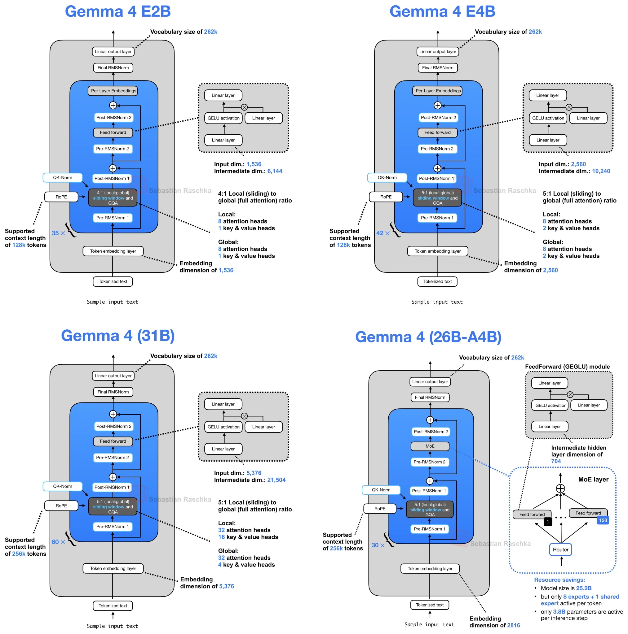
Figure 2: Gemma 4 architecture drawings.
The first small architecture tweak in the E2B and E4B variants is that they adopt a shared KV cache scheme, where later layers reuse key-value states from earlier layers to reduce long-context memory and compute.
Before explaining KV-sharing further, let’s briefly talk about the motivation. As I wrote and talked about in recent months, one of the main recent themes in LLM architecture design is KV cache size reduction. In turn, the motivation behind KV cache size reduction is to reduce the required memory, which allows us to work with longer contexts, which is especially relevant in the age of reasoning models and agents. For more background on KV caching, see my “Understanding and Coding the KV Cache in LLMs from Scratch” article:
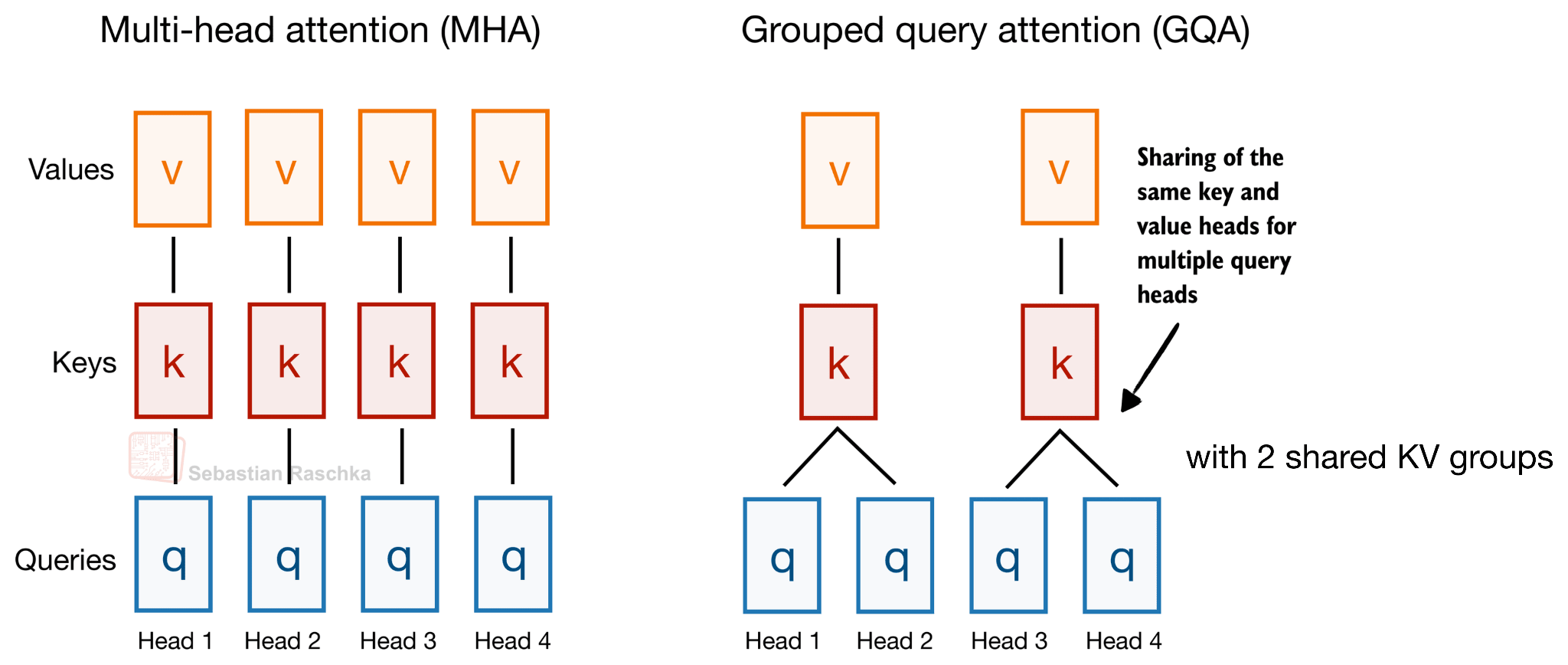
To pick a classic example (that Gemma 4 still uses): Grouped Query Attention (GQA) already shares key-value (KV) heads across different query heads to reduce the KV cache size, as illustrated in the figure below.
Figure 3: Grouped Query Attention (GQA) shares the same key (K) and value (V) heads among multiple query (Q) heads.
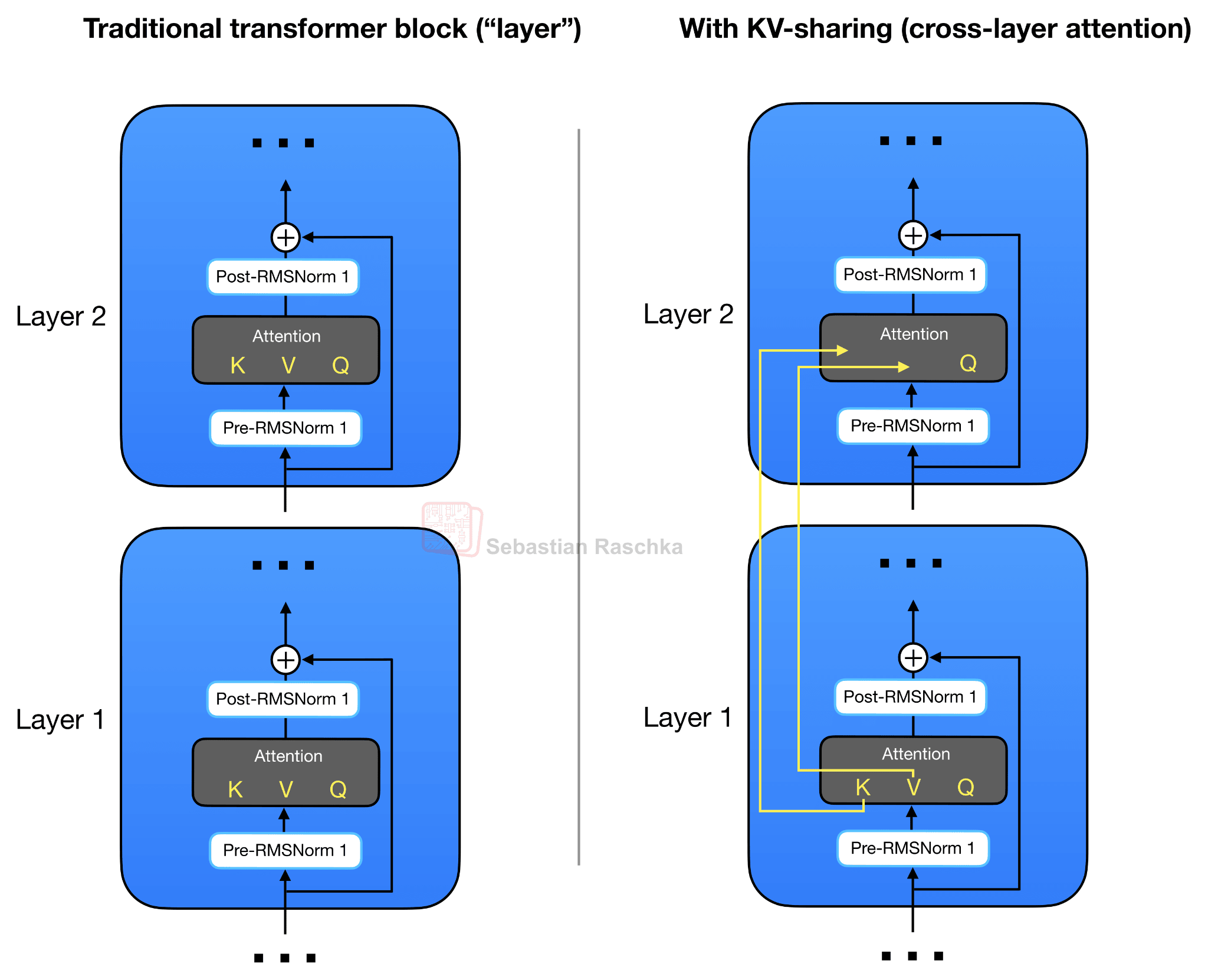
As mentioned before, Gemma 4 uses GQA. However, in addition to the KV sharing among queries as part of GQA, Gemma 4 also shares KV projections across different layers instead of computing it as part of the attention module in each layer. This KV-sharing scheme, also called cross-layer attention, is illustrated in the figure below.
Figure 4: Regular transformer blocks compute separate Q, K, and V projections in each attention module (left). Cross-layer attention designs (right) share the same K and V projections across multiple layers.
As briefly hinted at in the architecture overview in Figure 2, Gemma 4 E2B uses regular GQA and sliding window attention in a 4:1 pattern. (More precisely, Gemma 4 E2B uses MQA, which is the one-KV-head special case of GQA).
In the case of GQA (or MQA), the KV-sharing works like this. Later layers no longer compute their own key and value projections but reuse the KV tensors from the most recent earlier non-shared layer of the same attention type. In other words, sliding-window layers share KV with a previous sliding-window layer. Full-attention layers share KV with a previous full-attention layer. The layers still compute their own query projections, so each layer can form its own attention pattern, but the expensive and memory-heavy KV cache is reused across several layers.
For example, Gemma 4 E2B has 35 transformer layers, but only the first 15 compute their own KV projections; the final 20 layers reuse KV tensors from the most recent earlier non-shared layer of the same attention type. Similarly, Gemma 4 E4B has 42 layers, with 24 layers computing their own KV and the final 18 layers sharing them.
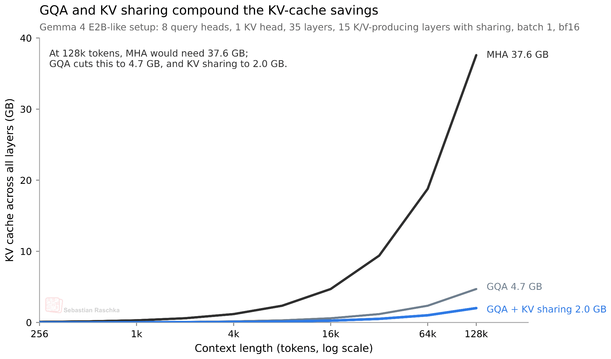
How much does this actually save? Since we share roughly half of the KVs across layers, we save approximately half of the KV cache size. For the smallest E2B model, this results in a 2.7 GB saving (at bfloat16 precision) in long 128K contexts, as shown below. (For the E4B variant, this saves about 6 GB at 128K.)
Figure 5: KV cache memory savings from GQA and cross-layer KV sharing in a Gemma 4 E2B-like setup. For simplicity, additional savings from sliding window attention are not shown.
The downside of KV-sharing is, of course, that it’s an “approximation” of the real thing. Or, more precisely, it reduces model capacity. However, according to the cross-layer attention paper, the impact can be minimal (for small models that were tested).
2. Per-Layer Embeddings and “Effective” Size (Gemma 4 E2B/E4B)
The Gemma 4 E2B and E4B variants include a second efficiency-oriented design choice called per-layer embeddings (PLE). This is separate from the KV-sharing scheme above.
KV sharing reduces the KV cache. PLE is instead about parameter efficiency, where it lets the small Gemma 4 models use more token-specific information without making the main transformer stack as expensive as a dense model with the same total parameter count.
For instance, the “E” in Gemma 4 E2B and E4B stands for “effective”. Concretely, Gemma 4 E2B is listed as 2.3B effective parameters, or 5.1B parameters when the embeddings are counted. (Similarly, Gemma 4 E4B is listed as 4.5B effective parameters, or 8B parameters with embeddings).
In short, in the “E” models, the main transformer-stack compute is closer to the smaller number, while the larger number includes the additional embedding-table layers. (For an illustration of how embedding layers work, see my “Understanding the Difference Between Embedding Layers and Linear Layers” code notebook.)
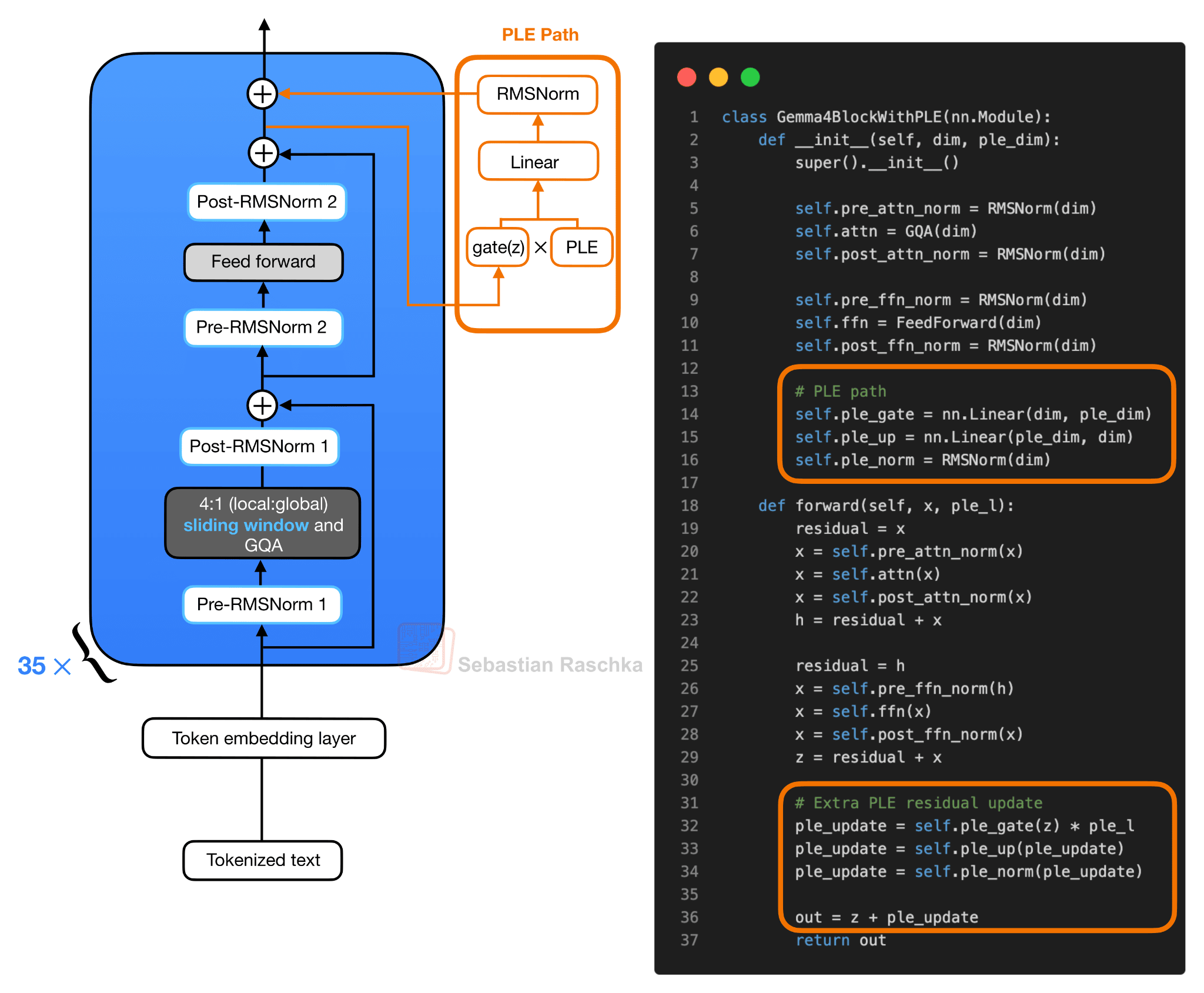
Conceptually, the new PLE path looks like this:
Figure 6: Simplified Gemma 4 block with the PLE residual path. The normal block first computes the attention and feed-forward residual updates. The resulting hidden state gates the layer-specific PLE vector, and the projected PLE update is added as an extra residual update at the end of the block.
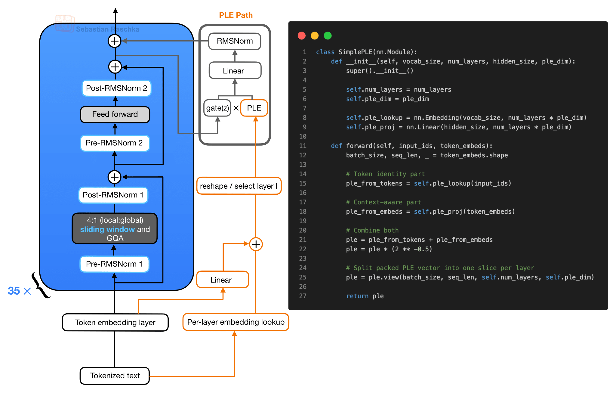
The PLE vectors themselves are prepared outside the repeated transformer blocks. In simplified form, there are two inputs to the PLE construction. First, the token IDs go through a per-layer embedding lookup. Second, the normal token embeddings go through a linear projection into the same packed PLE space. These two pieces are added, scaled, and reshaped into a tensor with one slice per layer. Note that each block then receives its own slice.
Figure 7: Simplified PLE construction. The token IDs provide a per-layer embedding lookup, while the normal token embeddings are projected into the same space. The two contributions are combined and reshaped so that each transformer block receives its own layer-specific PLE slice.
The important detail is that PLE does not give each transformer block a full independent copy of the normal token embedding layer. Instead, the per-layer embedding lookup is computed once. Then, as mentioned before, it gives each layer a small token-specific embedding slice (via “reshape / select layer l”.
So, for each input token, Gemma 4 prepares a packed PLE tensor that contains one small vector per decoder layer. Then, during the forward pass, layer l receives only its own slice (ple_l in the Gemma4WithPLEBlock in figure 6).
Inside the transformer block, the regular attention and feed-forward branches run as usual. First, the block computes the attention residual update. Then it computes the feed-forward residual update. After that second residual add, the resulting hidden state, which I denoted as z in the pseudocode in figure 6, is used to gate the layer-specific PLE vector. The gated PLE vector is projected back to the model hidden size, normalized, and added as one extra residual update.
So the useful mental model is that the transformer block still has the same main attention and feed-forward path, but Gemma 4 adds a small layer-specific token vector after the feed-forward branch. This increases representational capacity through embedding parameters and small projections. This adds computational overhead but avoids the cost of scaling the entire transformer stack to the larger parameter count.
But why PLEs? The simpler alternative would be to make the dense model smaller, using fewer layers, narrower hidden states, or smaller feed-forward networks. That would reduce memory and latency, but it also removes capacity from the parts of the model that do the main computation.
The PLE design keeps the expensive transformer blocks closer to the smaller “effective” size, while storing additional capacity in per-layer embedding tables. These are much cheaper to use than adding more attention or FFN weights, since they are mainly lookup-style parameters that can be cached.
Also, we have to take Google’s word here that this is an effective and worthwhile design choice. It would be interesting to see some comparison studies to see how this E2B design compares to a regular Gemma 4 2.3B model and a regular Gemma 4 5.1B model.
Also, in principle, PLE is not inherently limited to small models. We could attach per-layer embedding slices to larger models, too. However, larger models already have sufficient capacity where these extra embeddings may not help that much. Also, for larger models, we already use MoE designs as a trick to increase capacity while keeping the compute footprint smaller.
By the way, if you are interested in a relatively simple and readable code implementation, I implemented the Gemma 4 E2B and E4B models from scratch here.
Laguna is the first open-weight model by Poolside, a Europe-based company focused on training LLMs for coding applications. Several of my former colleagues joined Poolside in recent years, and they have a great team with lots of talent. It’s just nice to see more companies also releasing some of their models as open-weight variants.
Anyways, the Laguna XS.2 architecture depicted below looks very standard at first glance. However, one detail that I didn’t show (/try to cram into there) is a concept we can refer to as “Layer-wise attention budgeting”.
Figure 9: Poolside’s Laguna XS.2 architecture.
Part of the idea behind the attention budgeting here is that instead of giving every transformer layer the same full attention budget, Laguna XS.2 varies the attention cost by layer. It has 40 layers total, with 30 sliding-window attention layers and 10 global/full attention layers. As usual, the sliding-window layers only attend over a local window (here: 512 tokens), which keeps the KV cache and attention computation cheaper. The global layers are more expensive but preserve the ability to access all information in the context window.
This mixed sliding-window + global/full attention pattern is not unique to Laguna XS.2 and is used by many other architectures (including Gemma 4).
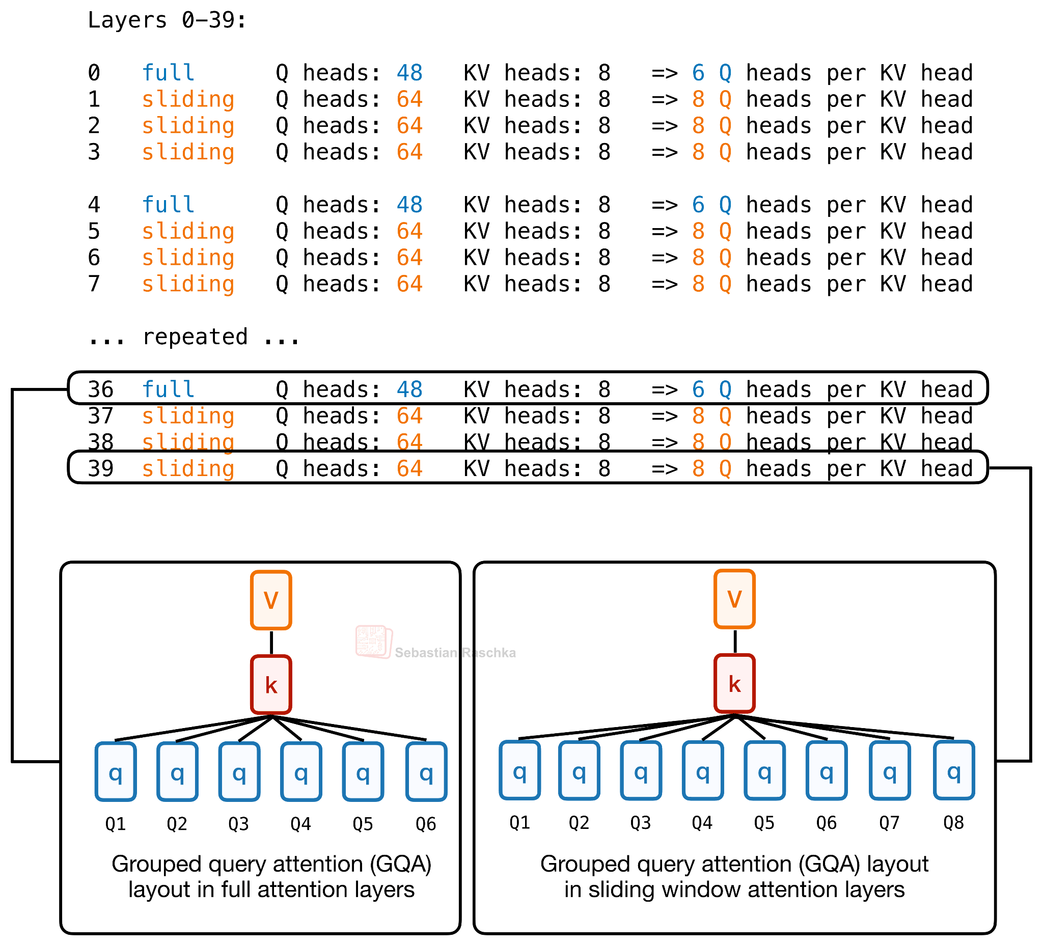
But what’s new is the use of per-layer query-head counts. For instance, the Hugging Face model hub config.json includes a num_attention_heads_per_layer setting, so layers can have different numbers of query heads while keeping the KV cache shape compatible.
Figure 10: Per-layer query-head budgeting in Laguna, where full attention layers use 6 query heads per KV head, and sliding window attention layers use 8 query heads per KV head.
So Laguna XS.2 gives more query heads to sliding-window layers and fewer query heads to global layers, while keeping the KV heads fixed at 8. That is the actual layer-wise head budgeting in the config.
Laguna XS.2 is one of the most prominent recent examples of this per-layer query-head budgeting in a production-style open model. But the broader idea of varying model capacity by layer goes back to (at least) Apple’s 2024 OpenELM.
And again, what’s the point of such a design? Similar to KV-sharing, the point is to spend attention capacity where it is most useful, instead of giving every layer the same budget. Specifically, full-attention layers are expensive because they look across the whole context, so Laguna gives them fewer query heads compared to sliding window attention modules.
(Besides, another smaller implementation detail is that Laguna also applies per-head attention-output gating; this is somewhat similar to Qwen3-Next and others, which I also omit here since I covered it in earlier articles.)
4. Compressed Convolutional Attention (ZAYA1-8B)
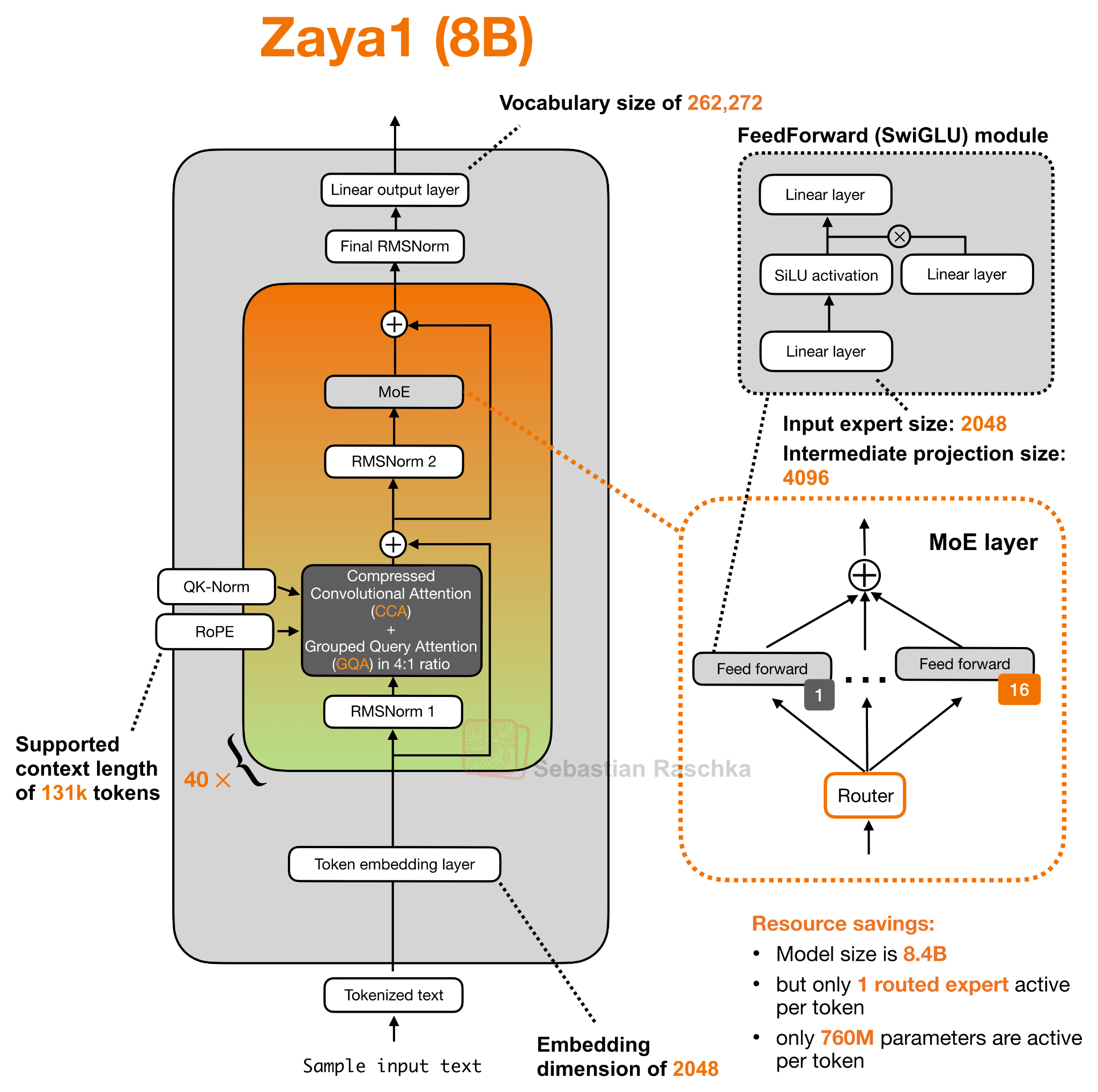
Similar to Laguna, ZAYA1-8B is another new player on the open-weight market. It is developed by Zyphra, and one of the interesting details around the release is that the model was trained on AMD GPUs rather than the more common NVIDIA GPU (or Google TPU) setup.
The main architecture detail, though, is Compressed Convolutional Attention (CCA), used together with grouped-query attention. Unlike MLA-style designs that mainly use a latent representation as a compact KV cache format, CCA performs the attention operation directly in the compressed latent space, but more on that later.
(Sidenote: the ZAYA1-8B config.json lists 80 alternating layer entries rather than 40 conventional transformer blocks. These entries alternate between CCA/GQA attention and MoE feed-forward layers. But for the architecture figure, it is more convenient to visualize this as 40 repeated attention + MoE pairs, which is conceptually equivalent.)
As hinted at in the figure above, ZAYA1-8B uses Compressed Convolutional Attention (CCA) together with a 4:1 GQA layout. The key point is that its attention block is built around CCA rather than a standard sliding-window attention block.
What is Compressed Convolutional Attention?
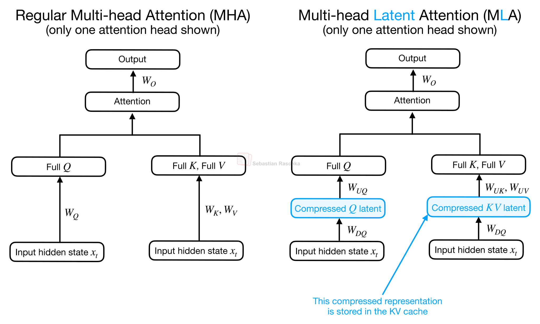
I would say CCA is related in spirit to Multi-head Latent Attention (MLA) in DeepSeek’s models, since both introduce a compressed latent representation into the attention block. However, they use that latent space differently. MLA mainly uses the latent representation to reduce the KV cache. In MLA, the KV tensors are stored compactly and then projected into the attention-head space for the actual attention computation.
Figure 12: Regular Multi-head Attention (MHA) and Multi-head Latent (MLA) attention side by side.
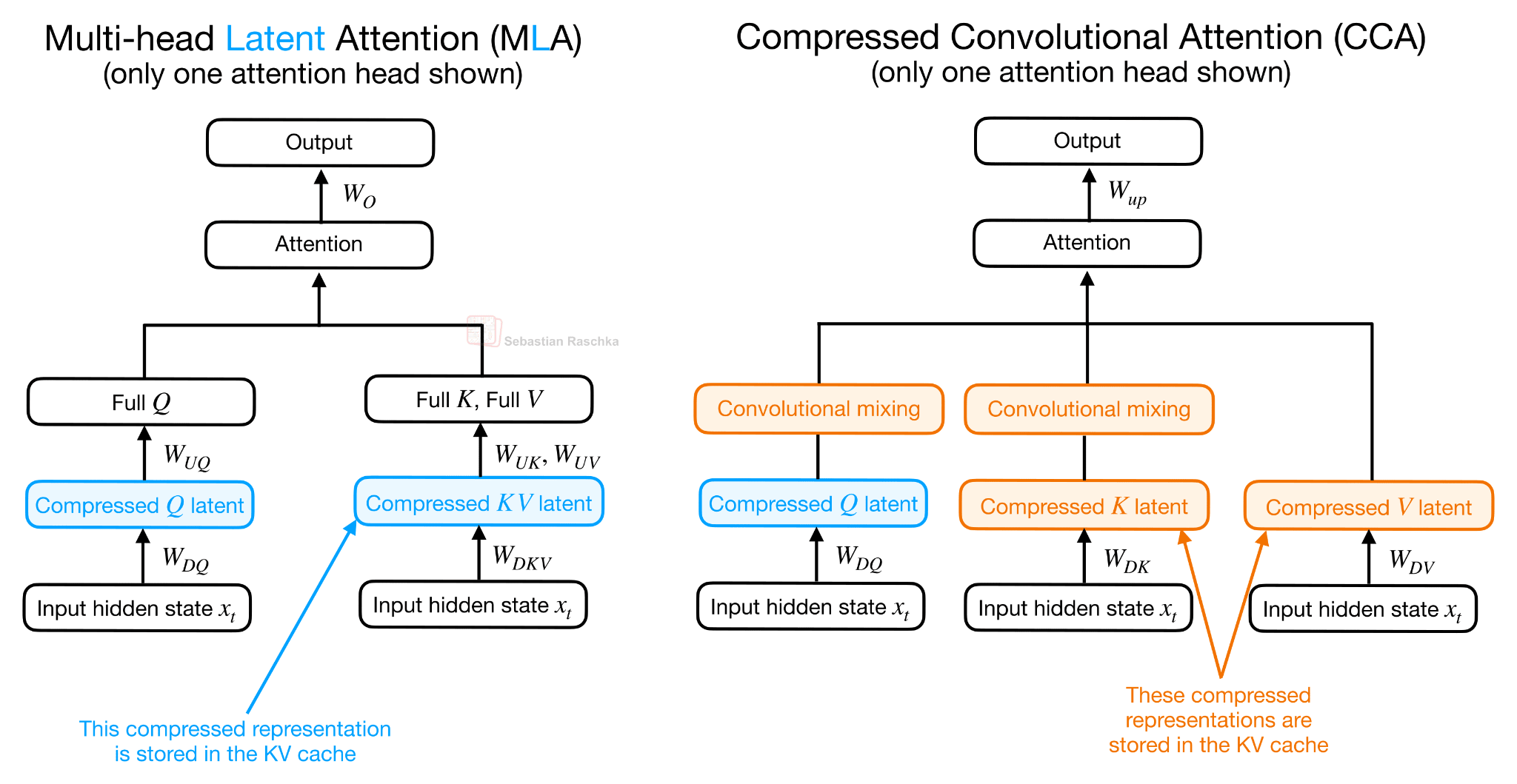
CCA compresses Q, K, and V and performs the attention operation directly in the compressed latent space. This is why CCA can reduce not only KV cache size, but also attention FLOPs during prefill and training.
Figure 13: Multi-head Latent Attention (MLA) and Compressed Convolutional Attention (CCA) side by side.
As Figure 13 above illustrates, in CCA, the compressed, latent representations enter the attention mechanism directly, and the resulting compressed attention vector is then up-projected.
Note that this is called Compressed Convolutional Attention, not just Compressed Attention, since there is an additional convolutional mixing happening on the latent K and Q representations. The convolutional mixing part is not shown in Figure 12, because it would have been too crammed, but it’s relatively straightforward.
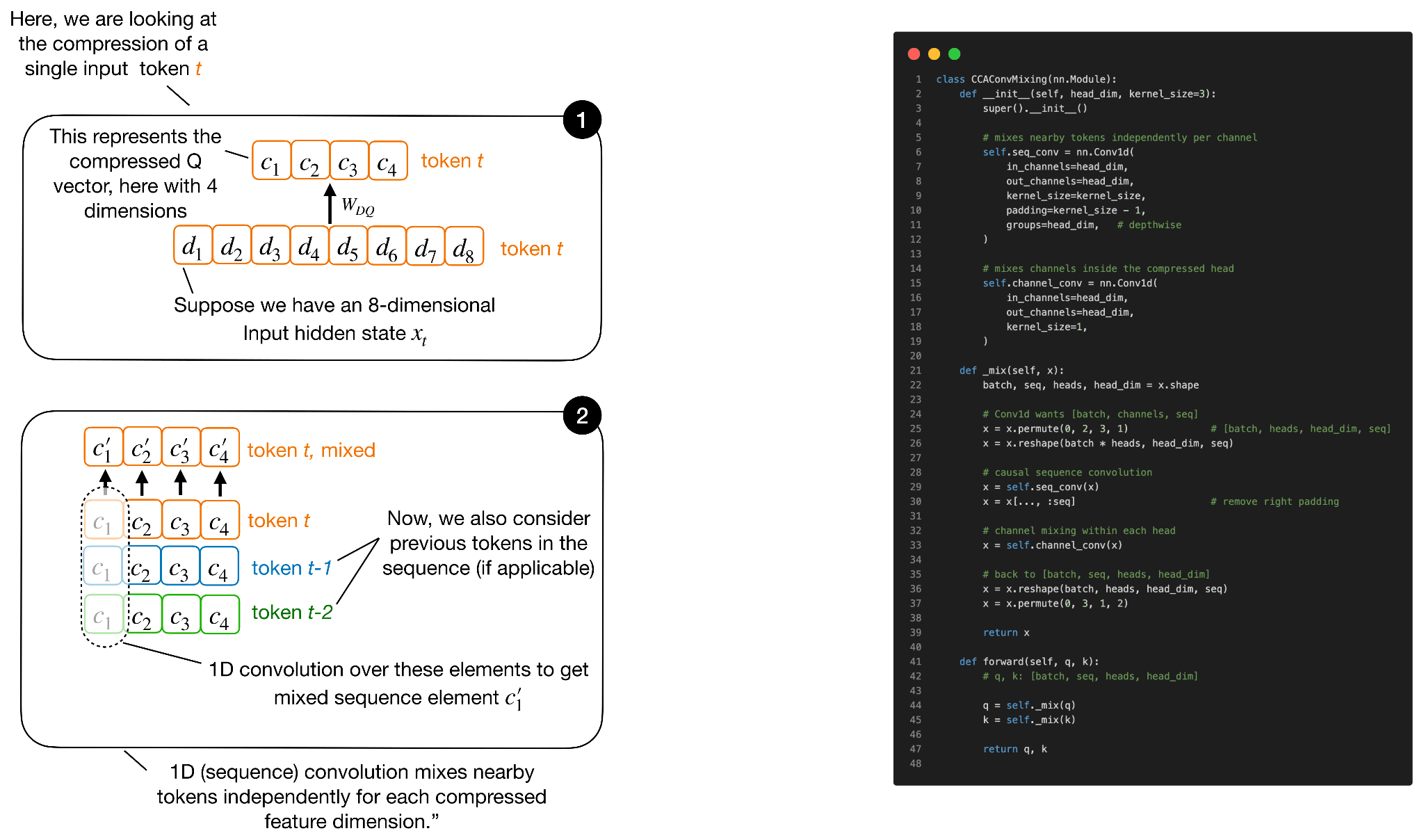
As hinted at in Figure 13, the convolutional mixing happens directly on the compressed Q and K tensors. The point is that compression makes Q, K, and V narrower, which saves compute and cache, but it can also make attention less expressive. The convolutions are a cheap way to give the compressed Q and K vectors more local context before they are used to compute attention scores. (The convolutional mixing is only applied to Q and K, not V, because Q and K determine the attention scores, while V represents the content that gets averaged via these scores).
Figure 14: conceptual overview of the sequence-mixing convolution
Next to the sequence mixing shown in Figure 14, there is also a channel mixing component. It’s in principle similar though, so I am omitting the illustration.
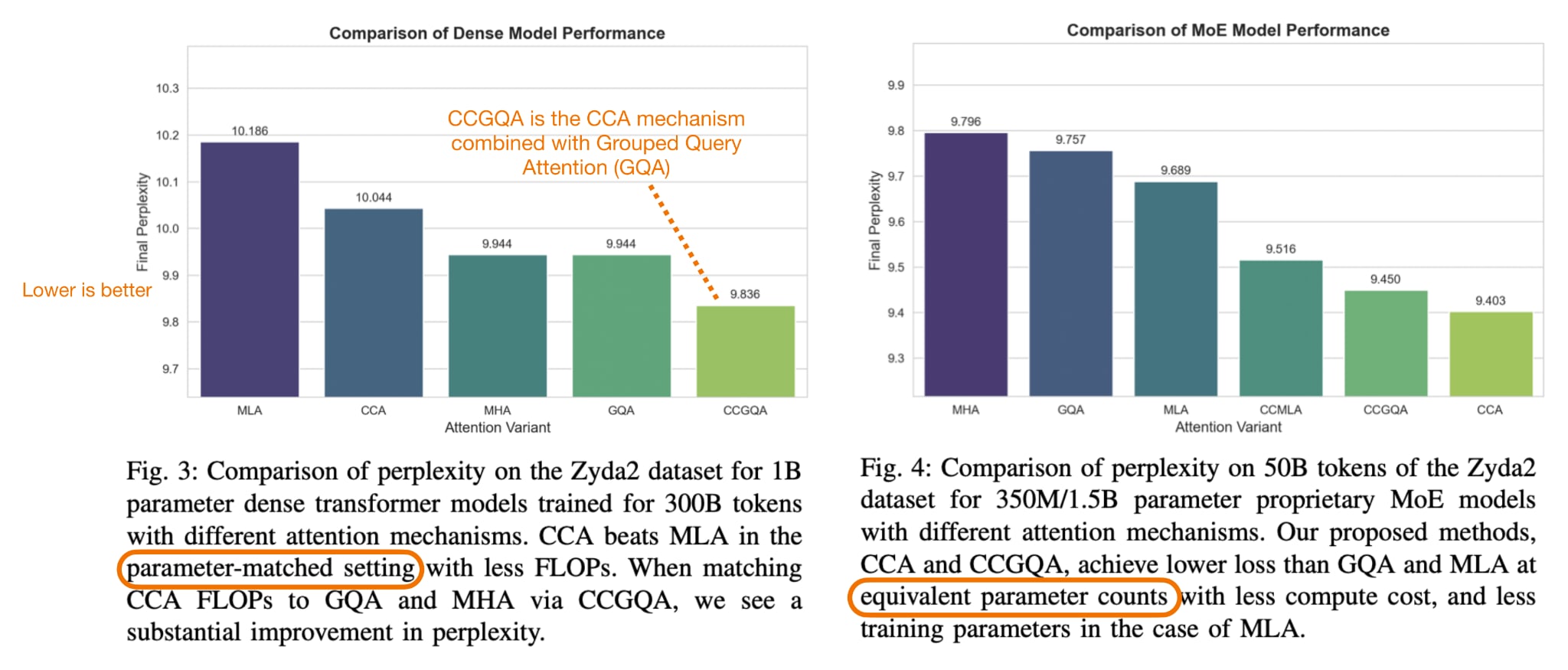
But the question is, “is it better than MLA”? According to the CCA paper’s own experiments, yes, they report CCA outperforming MLA under comparable compression settings.
Overall, the interesting part here is really the new attention mechanism. The model also uses a pretty extreme (= very sparse) MoE setup, with only one routed expert active per token, but that part is more familiar. CCA is more unusual because it performs the attention operation directly in a compressed latent space, and then uses convolutional mixing on the compressed Q and K representations to make this compressed attention less limiting. So, in short, ZAYA1-8B is not only trying to save compute in the feed-forward layers, but also in the attention mechanism itself.
5. CSA/HCA, mHC, and Compressed Attention Caches (DeepSeek V4)
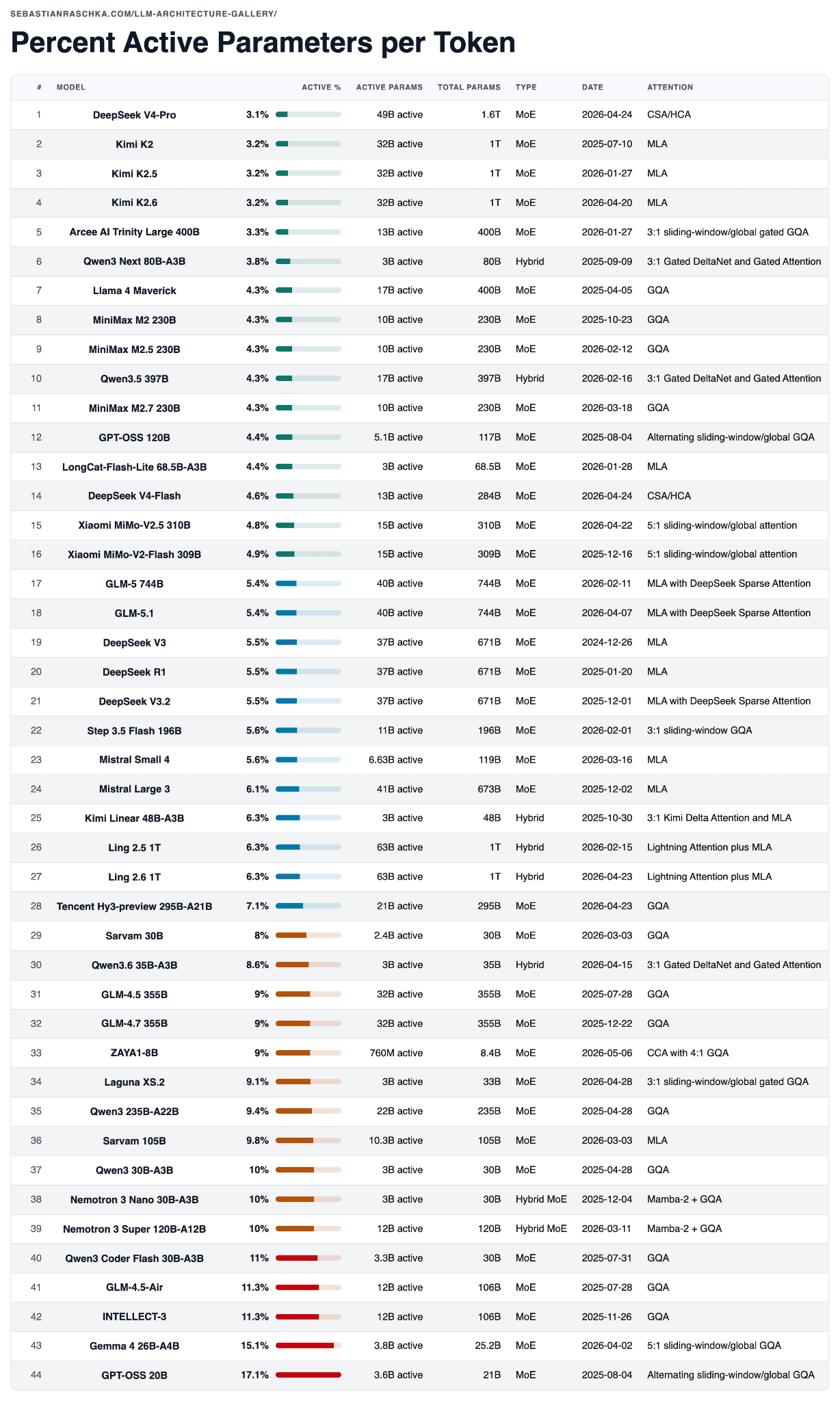
DeepSeek V4 was the biggest release of the year so far, both in terms of hype and model size. Interestingly, DeepSeek V4-Pro is also the most parameter-sparse MoE among the models in the table below, measured by active-parameter share, as summarized in the table below.
Caveat: active parameter share is only one lens. It does not capture KV cache size, attention pattern, context length, routing overhead, hardware efficiency, or training quality. But it is a helpful, quick check when comparing sparse models.
There’s a lot to say about DeepSeek V4, but since it’s been all over the news already, and to stay on topic regarding architecture tweaks, I will focus on the two most relevant parts that are new compared to previous architectures:
mHC for a wider residual pathway,
CSA/HCA for long-context attention compression and sparsity
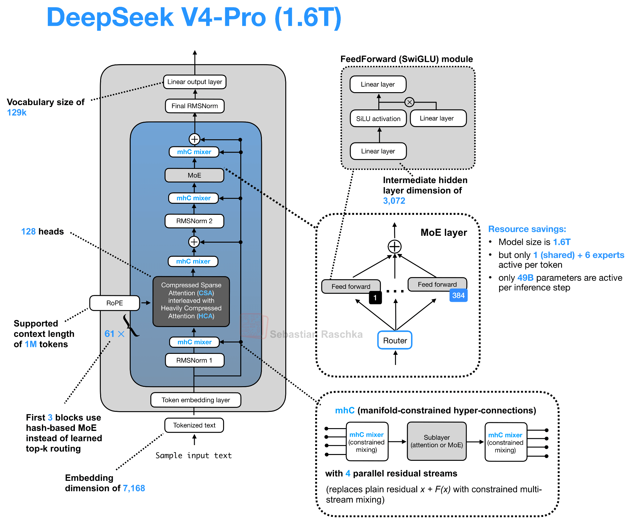
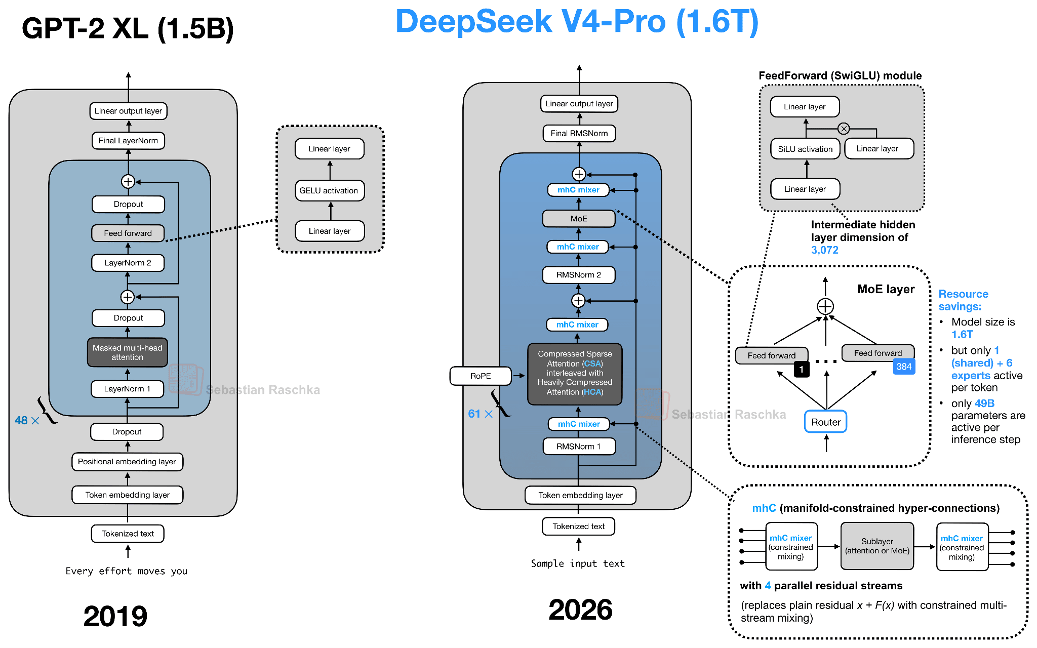
Looking at the DeepSeek V4 architecture drawing below, there seems to be a lot going on. The useful way to read it is to separate the residual-path change, mHC, from the attention-path changes, CSA/HCA, and compressed attention caches.
Figure 17: DeepSeek V4-Pro architecture overview.
5.1 Manifold-Constrained Hyper-Connections (mHC)
Let’s start with the mHC component of DeepSeek V4. This goes back to a research paper that the DeepSeek team shared last year (31 Dec 2025, mHC: Manifold-Constrained Hyper-Connections). However, in this paper, the technique was only tested on an experimental 27B scale model. Now, we see it in their flagship release, which is a good sign that this idea actually works well in production.
The main idea behind mHC here is to modernize the design of the residual connections inside the transformer block, which is refreshing, because architecture tweaks are usually focused on the attention mechanism, normalization layer placement, and MoE parts.
Now, mHC is based on previous work on hyper-connections (see Hyper-connections by Zhu et al., 2024), which we should briefly discuss first. Hyper-connections essentially modify the single residual stream inside the transformer block by replacing it with several parallel residual streams and learned mappings between them.
(For those new to residual connections, I made a video on residual neural networks many years ago, where I explained the general mechanism.)
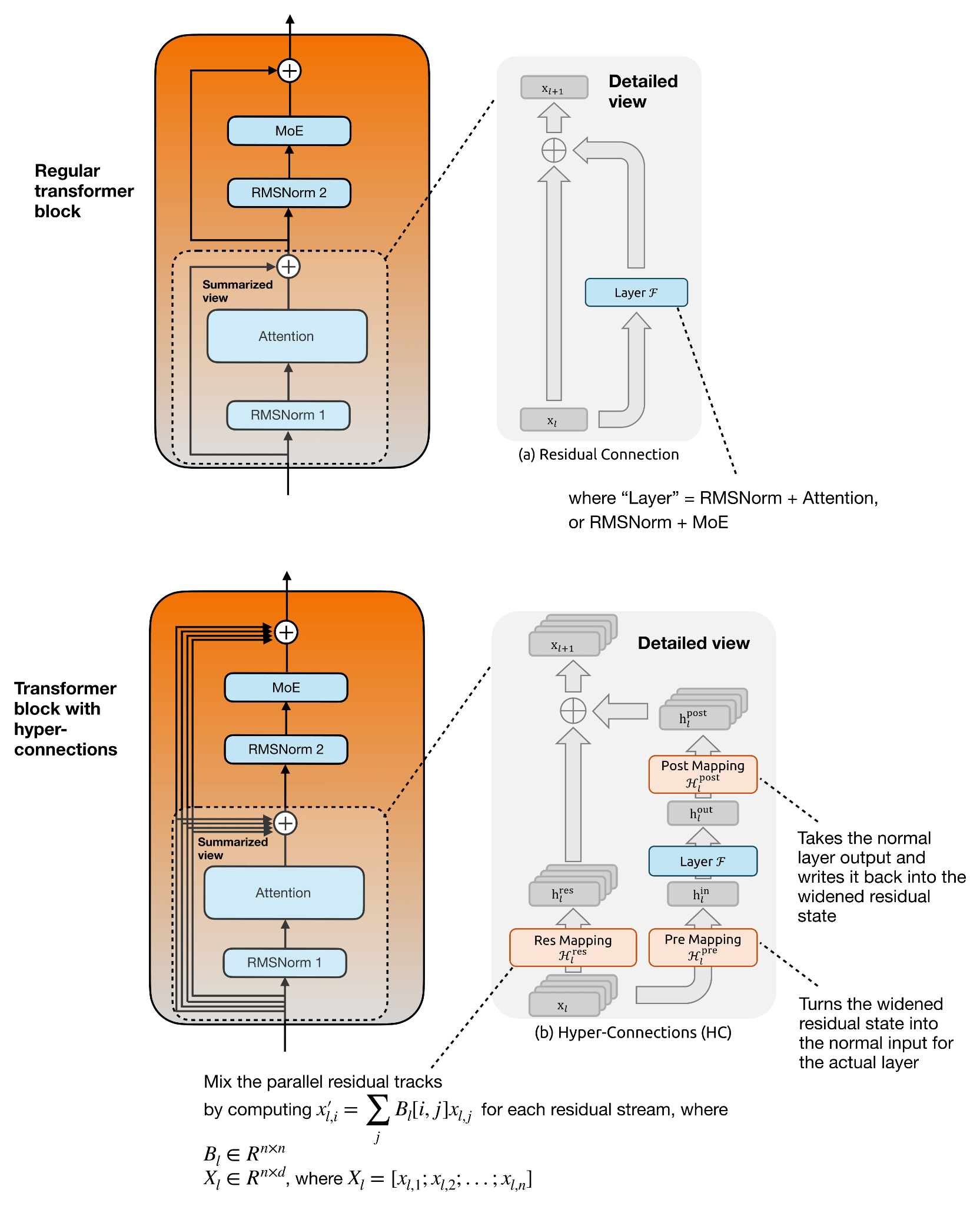
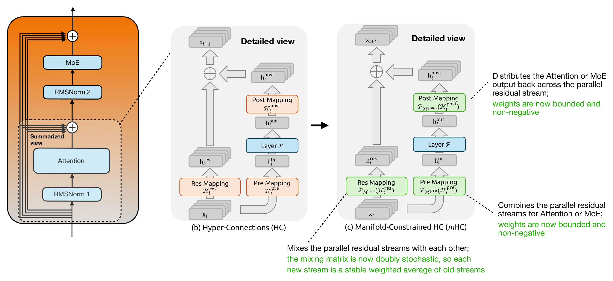
The idea behind hyper-connections is to widen the residual stream. We can think of this as keeping several parallel residual streams, with an additional Res Mapping linear transformation that mixes them across layers. Since the Attention or MoE layer itself still operates on the normal hidden size, hyper-connections also add a Pre Mapping that combines the parallel residual streams into one normal hidden vector for the layer, and a Post Mapping that distributes the layer output back across the parallel residual streams. This is visually summarized in the figure below.
Figure 18: Regular transformer block (top) vs transformer block with hyper-connections (bottom) using annotated figures from the mHC paper, https://arxiv.org/abs/2512.24880.
The figure below focuses on the attention-layer portion of the transformer block, but the same concept applies to the second residual branch around the MoE layer.
The purpose of hyper-connections is to make the residual pathway more expressive without making the actual Attention or MoE layer wider. This is only mildly more expensive in FLOPs because the extra mappings operate over the small residual-stream axis, for example, n = 4 in DeepSeek V4, not over a huge hidden dimension.
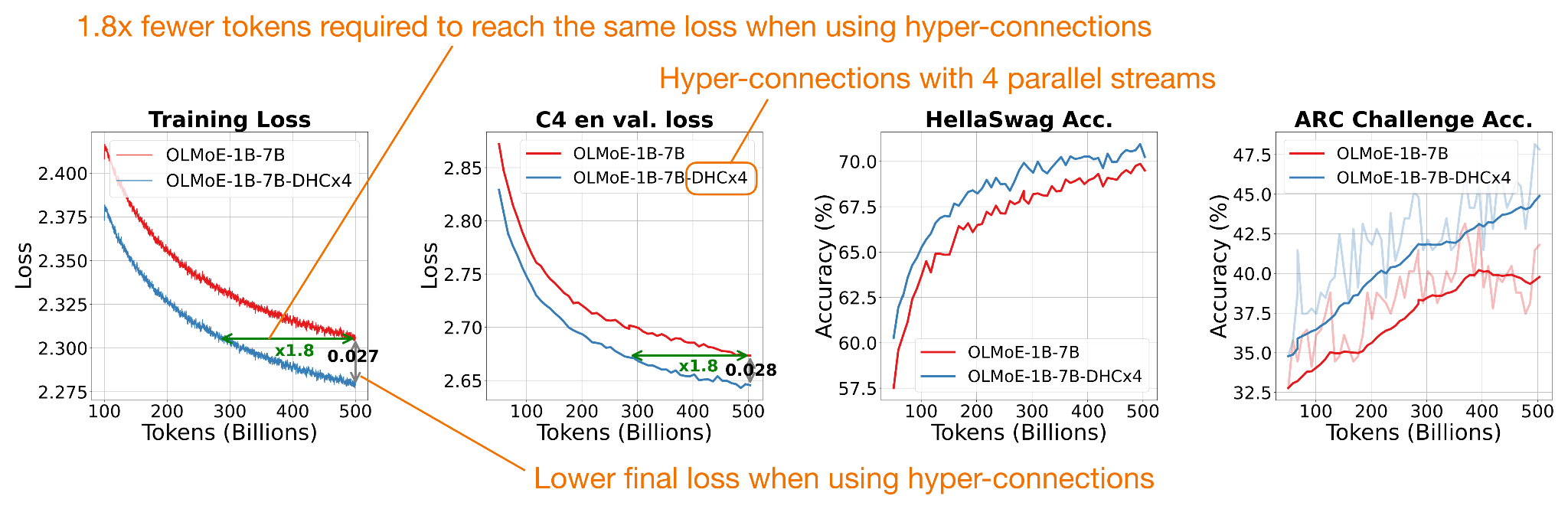
In the original hyper-connections paper, the 7B OLMo MoE experiment goes from 13.36G to 13.38G FLOPs per token, which is basically unchanged. In terms of reported gains, there were modest (but consistent) improvements, as shown in the figure below.
(However, only looking at FLOPs is a bit simplistic. The widened residual state still has to be stored, moved through memory, mixed, etc. So the practical overhead can come more from memory traffic and implementation complexity than from arithmetic, which is not explicitly measured. However, given that DeepSeek V4 is all about efficiency, it seems to be a worthwhile addition.)
Figure 19: Hyper-connections performance versus baseline, using an annotated figure from the hyper-connections paper, https://arxiv.org/abs/2409.19606.
Also, as shown in the figure above, metrics reached the baseline’s performance using roughly half the training tokens.
The main change from regular hyper-connections (HC) to manifold-constrained hyper-connections (mHC) is that the mappings are no longer left unconstrained. In regular HC, the Res Mapping is a learned matrix that mixes the parallel residual streams, but stacking many such matrices can amplify or shrink signals unpredictably.
In mHC, this residual mapping is projected onto the manifold of doubly stochastic matrices, meaning all entries are non-negative and each row and column sums to 1. This makes the residual mixing behave more like a stable redistribution of information across streams. The Pre Mapping and Post Mapping are also constrained to be non-negative and bounded, which avoids cancellation when reading from and writing back into the widened residual state. In short, mHC keeps the richer residual mixing of HC, but adds constraints so it scales more safely, which becomes more relevant for larger (deeper) models.
Otherwise, the main idea of using parallel residual streams remains, as shown in the figure below.
Figure 20: Transformer block with hyper-connections (HC) and manifold-constrained hyper-connections (mHC) using annotated figures from the mHC paper, https://arxiv.org/abs/2512.24880.
In the mHC paper, using a 27B parameter model for the experiments, the DeepSeek team’s optimized implementation (with fusion, recomputation, and pipeline scheduling) adds only 6.7% additional training time overhead for 4 residual streams (n = 4) throughout all transformer blocks compared to the single-stream baseline.
To sum up this section, HC/mHC changes how information is carried around these layers by replacing the single residual stream with several interacting residual streams, with the additional stability constraints added in mHC, while adding minimal compute overhead. Also, it pairs well with the CSA/HCA attention changes, which modify other parts of the transformer block, which I will discuss below.
5.2 Compressed Attention via CSA and HCA
The other major DeepSeek V4 architecture change is on the attention side. Again, the motivation is that at very long context lengths, attention becomes expensive not only because of the attention score computation, but also because the KV cache grows with the sequence length. DeepSeek V4 addresses this issue with a hybrid of two compressed-attention mechanisms, Compressed Sparse Attention (CSA) and Heavily Compressed Attention (HCA).
For a refresher, I recommend checking out my previous “A Visual Guide to Attention Variants in Modern LLMs” article, which covers Multi-head Latent Attention (MLA) and DeepSeek Sparse Attention (DSA), among others.
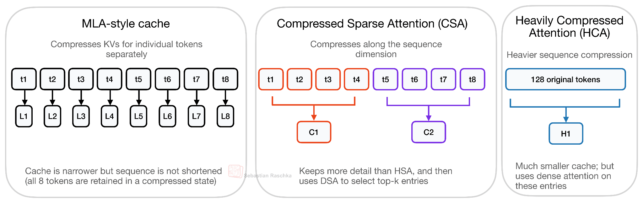
The first thing to note is that CSA/HCA in DeepSeek V4 is a different kind of compression than the MLA-style compression used in DeepSeek V2/V3. Where MLA mainly compresses the per-token KV representation, CSA and HCA compress along the sequence dimension. So, instead of keeping one full (or compressed) KV entry for every previous token, they summarize groups of tokens into fewer compressed KV entries. Consequently, the cache gets shorter. DeepSeek V4 also uses compact compressed entries and shared-KV attention, but the main distinction from MLA is the sequence-length compression. This is illustrated in the figure below.
Figure 21: Conceptual comparison of MLA-style per-token latent caching, CSA, and HCA. MLA compresses the stored KV representation but keeps one latent entry per token. CSA shortens the sequence more mildly with m=4 and sparse top-k selection, while HCA uses much heavier sequence compression with m’=128 and dense attention over the shorter cache.
The quality tradeoff for CSA/HCA is also different from MLA. As shown in the figure above, MLA compresses the representation stored for each token, but it still keeps one latent KV entry per token. CSA and especially HCA go further by reducing the number of sequence entries themselves, so the model gives up some token-level info in exchange for much lower long-context cost.
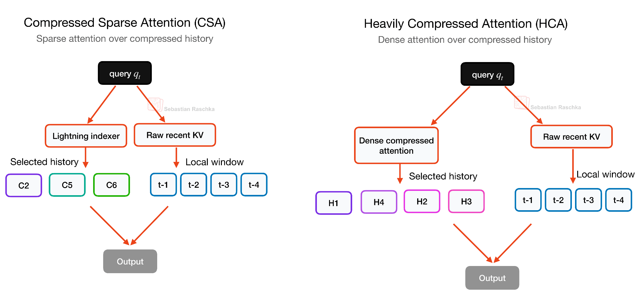
Again, it’s all about reducing long-context cost, but this trade-off can hurt modeling quality if the compression is too strong, which is why DeepSeek V4 does not rely on one compression scheme alone but alternates between CSA and HCA. CSA uses a milder compression rate and a DeepSeek Sparse Attention (DSA)-style selector, HCA uses much heavier compression for cheaper global coverage, and both keep a local sliding-window branch for recent uncompressed tokens. This sparse selection in CSA builds on DeepSeek Sparse Attention (DSA), which I discussed in more detail in my earlier DeepSeek V3.2 write-up.
HCA is the more aggressive variant of the two. It compresses every 128 tokens into one compressed KV entry, but then uses dense attention over those heavily compressed entries. In other words, CSA keeps more details but uses sparse selection, while HCA keeps far fewer entries and can afford dense attention over them, as illustrated in the figure below. This makes the two mechanisms somewhat complementary, which is why DeepSeek V4 interleaves CSA and HCA layers rather than using only one of them.
Figure 22: CSA selects a sparse set of compressed history blocks, while HCA attends densely over more heavily compressed blocks. Both paths also include recent uncompressed KV entries through a 128-token sliding-window branch.
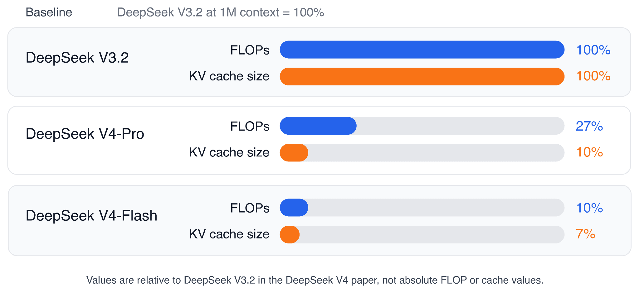
The DeepSeek V4 paper reports that, at a 1M-token context length, DeepSeek V4-Pro uses only 27% of the single-token inference FLOPs and 10% of the KV cache size compared with DeepSeek V3.2, which uses MLA and DeepSeek Sparse Attention (DSA). DeepSeek V4-Flash is even smaller, at 10% of the FLOPs and 7% of the KV cache size relative to DeepSeek V3.2.
Figure 23. Reported 1M-context efficiency numbers from the DeepSeek V4 paper, relative to DeepSeek V3.2.
By the way, I would not describe CSA/HCA as “better” than MLA in a general sense. CSA/HCA is a more aggressive long-context design. And it’s also more complicated for sure. Unfortunately, there is no ablation study in the paper. But overall, the paper reports strong overall modeling results, including DeepSeek V4-Flash-Base outperforming DeepSeek V3.2-Base on a majority of base-model benchmarks and strong 1M-token retrieval results, but these results are for the full DeepSeek V4 recipe, which also includes better data, Muon-based optimization, mHC, precision/storage optimizations, and training/inference-system changes.
Personally, for now, I would treat CSA/HCA as an efficiency-focused long-context design that appears to preserve modeling quality well in their large flagship model(s) but not necessarily universally better than MLA.
6. Conclusion
Overall, the interesting pattern this year is that most new open-weight models try to make long-context inference cheaper without just shrinking the model in terms of total parameters. For instance,
Gemma 4 reduces KV-cache memory with cross-layer KV sharing and adds capacity via per-layer embeddings.
Laguna XS.2 tweaks how much attention capacity each layer gets.
ZAYA1-8B moves attention into a compressed latent space.
DeepSeek V4 adds constrained residual-stream mixing and compressed long-context attention.
All of these tweaks add more complexity, which seems to be where LLM architecture is going right now.
My main takeaway is that the transformer block is still changing, but in fairly targeted ways. The basic recipe is still based on the original GPT decoder-only transformer architecture, but many parts are upgraded or replaced, and they get more specialized for longer contexts and more efficient inference, whereas the qualitative modeling performance seems largely driven by data quality (and quantity) and training recipes.
The question many of you asked me in the past is centered on when (or if) transformers are being replaced with something else. Of course, there are other designs like diffusion models, but transformers remain the status quo for state-of-the-art architecture releases.
However, with each increasing yearly release quarter, we get more and more tweaks. While it was possible to implement a basic transformer block in perhaps 50-100 lines of PyTorch code, these tweaks (esp. around the attention variants) probably 10x the code complexity. This is not an inherently bad thing as these tweaks reduce (not increase) runtime costs. However, it’s becoming increasingly difficult to gain a clear understanding of the individual components and their interactions.
Figure 24: The evolution from GPT-2 (2019) to DeepSeek V4-Pro (2026)
For instance, I am fairly certain that someone who is diving into LLM architectures for the first time will be totally overwhelmed when seeing the DeepSeek V4 source code. However, by starting with the original decoder-style LLM (GPT/GPT-2) and then gradually adding / learning about these new components one at a time, we can keep the learning effort manageable. The moral of the story, I guess, is to keep learning, one architecture at a time :).
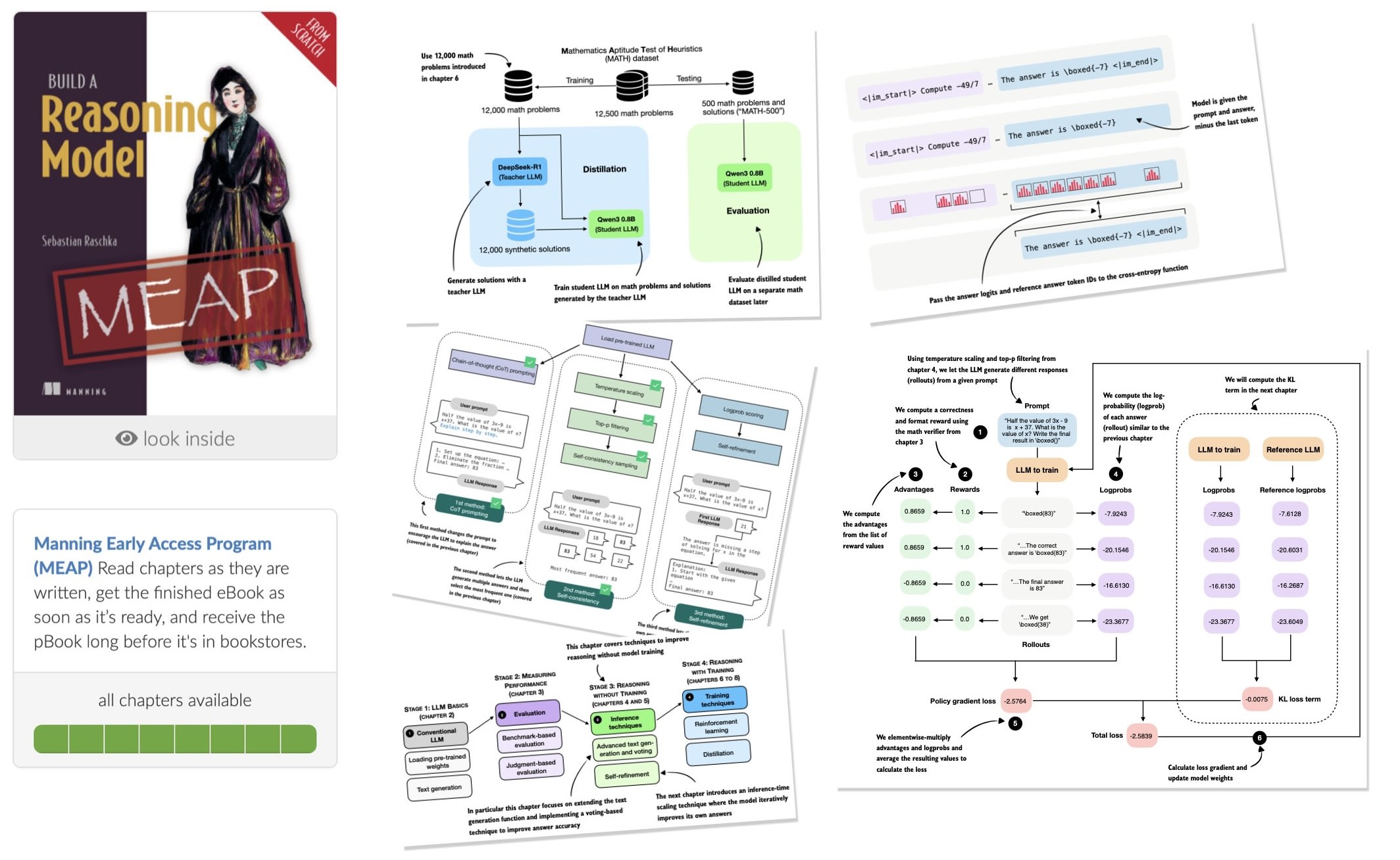
By the way, I am very excited to share that I finished writing Build A Reasoning Model (From Scratch) and all chapters are in early access now. The publisher and I worked hard on the final layouts in the past month, and it’s going to be send to the printer this week. (Good news: the print version will be in color this time!)
This is probably my most ambitious book so far. I spent about 1.5 years writing it, and a large number of experiments went into it. It is also probably the book I worked hardest on in terms of time, effort, and polish, and I hope you’ll enjoy it.
Build a Reasoning Model (From Scratch) on Manning and Amazon.
The main topics are
evaluating reasoning models
inference-time scaling
self-refinement
reinforcement learning
distillation
There is a lot of discussion around “reasoning” in LLMs, and I think the best way to understand what it really means in the context of LLMs is to implement one from scratch!
Amazon (pre-order of Kindle ebook and print paperback)
Video Friday is your weekly selection of awesome robotics videos, collected by your friends at IEEE Spectrum robotics. We also post a weekly calendar of upcoming robotics events for the next few months. Please send us your events for inclusion.
Bulk material handling is a critical, labor-intensive operation across various industries, traditionally performed by human operators using heavy hydraulic manipulators equipped with free-swinging, underactuated grippers. This work presents the first complete autonomous material-handling solution deployed on a real-world 40-ton material handler.
I don’t want to minimize this bedroom tidying by Figure (although I suppose I’m going to), but in the context of doing a task like this in place of a human, it really illustrates what these robots are comfortable with, and what they’re not.
Curious about what happens when street dance meets embodied AI? From smooth choreography to dynamic flips, NIX is exploring movement, rhythm, and real-world interaction through embodied AI. We’ll make NIX available—FOR FREE!—to selected partners from global universities, robotics labs, and creative technologists.
We introduce and open-source the Unified Autonomy Stack, a novel solution for resilient autonomy across aerial and ground robot morphologies. The architecture combines multimodal perception, multibehavior planning, and multilayered safe navigation to deliver mission-level autonomy across diverse robot morphologies. It fuses lidar, radar, vision, and inertial sensing to enable robust localization and mapping, vision-language-based scene reasoning, multibehavior planning, and layered safety through map-based avoidance, deep learned policies, and control barrier functions. The system supports Global Navigation Satellite System–denied navigation in perceptually degraded environments, exploration, object discovery, and inspection, and has been validated on multirotor and legged robots in challenging settings, demonstrating resilient performance.
Any robot doing anything consistently over a long period of time is impressive. Having said that, you want to be very careful about claiming that any robot operates at “human performance levels,” especially in a somewhat complex manipulation task, because humans are very, very good at stuff like this.
Robust.AI cofounder and CTO Rodney Brooks, ranked #44 on the Forbes 250 America’s Greatest Innovators list, sits down for a Q&A ahead of his panel discussion at the Forbes America Innovates event in San Francisco. We asked him two questions: What makes innovation in robotics such a challenge? What does the current surge in AI mean for robotics today?
This is one of the best robotic research videos I’ve ever seen—and don’t worry, according to the credits it’s not AI. And make sure to watch after the credits!
EFGCL is a guided-reinforcement learning method that efficiently enables highly dynamic motions through the use of assistive forces. In this work, we successfully achieved several dynamic motions, including jumping, backflips, and lateral flips.
Humanoid robots promise general-purpose assistance, yet real-world humanoid loco-manipulation remains challenging because it requires whole-body stability, dexterous hands, and contact-aware perception under frequent contact changes. In this work, we study dexterous, contact-rich humanoid loco-manipulation.
More than just technology, KATA Friends is a lifelike AI companion designed to see your world, feel your touch, and understand your heart. With expressive movements, evolving emotions, and natural conversations, Noa and Niko both grow alongside you to become a presence uniquely yours. From curious head tilts and playful reactions to ever-changing eye expressions and a soft, innocent voice, every interaction feels warm, personal, and alive.
One of the biggest challenges in robotics right now isn’t the hardware. It’s data. While many data-collection methods are effective, handheld data collection can create a diverse dataset of environments, conditions, and strategies for completing manipulation tasks. The Koala platform codesigned the handheld grippers and robot grippers around the same linkage mechanism, the same degrees of freedom, and the same force transmission. The human feels through the linkages what the robot will feel through its actuators.
Use ChatGPT for personal finance to connect your accounts, track spending and investments, manage subscriptions, create budgets, and plan financial goals.
Large language models (LLMs) keep getting bigger and better. But the cost of running them — generating text, answering questions, powering real-time applications — is scaling up, too. Obviously, model accuracy is important, but for real-time AI-based web applications, it can’t come at the expense of efficiency. In a paper we presented at the International Conference on Learning Representations (ICLR), we provide a framework for navigating this accuracy-versus-efficiency tradeoff, by connecting scaling laws directly to architectural-design decisions. The gap in current scaling laws In 2022, Google DeepMind announced the results of a study involving an experimental LLM called Chinchilla. The DeepMind researchers demonstrated a scaling law that enabled joint optimization of model size and training data to achieve a desired loss level, given a particular computational budget. More precisely, the law relates the model loss (L) to the number of model parameters (N) and the number of tokens in the training dataset: The other variables in this equation — E, A, B, α, and β — are all learnable coefficients. The DeepMind researchers did extensive experimentation to tune those coefficients. This "Chinchilla law" doesn't specify architectural choices, such as the size of the model's internal representations — the "hidden size" — or the relative number of parameters allocated to attention layers and multilayer perceptron (MLP) layers. However, two models, each with the same billion-parameter count, trained on the same data, with the same accuracy, can differ by up to 40% in inference-time throughput, depending on additional architectural choices. We set out to deduce scaling laws that can help predict those choices. The Transformer architecture The Transformer architecture — which lies at the heart of all LLMs — consists largely of stacked attention and MLP blocks. Attention blocks determine how much weight to give each prior token (word or word part) when updating the current token's representation; MLP blocks transform that representation further and are where much of the model's learned knowledge is stored. A separate output layer at the end of the stack converts the final representation into a probability distribution over the next token. The attention mechanism uses three matrices, with names borrowed from information retrieval: the query matrix encodes what each token is looking for in the rest of the sequence; the key matrix encodes what each token has to offer; and the value matrix holds the content each token can contribute when it's attended to. Comparing queries against keys tells the model how relevant each token is to each other token. Most LLMs use multihead attention: several attention computations run in parallel, each with its own query, key, and value projections. Different heads tend to specialize in different aspects of the input, letting the model capture a richer set of relationships than a single head would. Our approach: Architecture as a first-class variable In our ICLR paper, we introduce a scaling law that augments the Chinchilla framework with three architectural factors: the hidden size (the dimension of the vectors that flow through the embedding, attention, and MLP blocks); the ratio of the number of MLP parameters to the number of attention parameters; and grouped-query attention (GQA), in which groups of attention heads, while preserving distinct query matrices, share key and value matrices. Each factor has a direct impact on inference throughput: Hidden size (d_model): Under a fixed parameter budget, larger hidden sizes reduce total inference FLOPs and shrink the key-value cache, improving throughput. MLP-to-attention ratio (r_mlp/attn): A higher ratio allocates more parameters to the MLP and fewer to attention, shrinking the key-value cache and reducing memory-bandwidth bottlenecks. Grouped-query attention (GQA): Compressing key-value heads further cuts input/output costs during generation. Adjusting these factors purely for higher throughput comes at a cost of accuracy. Both hidden size and MLP-to-attention ratio exhibit U-shaped loss curves: there is an optimal point for each, and pushing too far in either direction has a negative effect on model accuracy. GQA has a more erratic effect on loss, so we treat it as a discrete hyperparameter tuned through local search. We deduce our scaling law in two stages. First, we fit the standard Chinchilla law to the model under investigation, calculating values for the coefficients E, A, B, α, and β. This establishes an optimal reference loss. Then we calibrate how each architectural choice — differences in the three factors we consider — affects that loss. Effectively, we learn a correction surface over the design space. Because the effects of hidden size and MLP-to-attention ratio on loss turn out to be separable, each factor can be optimized independently. Two model families: Panda and Surefire This scaling law enabled us to develop a search framework that identifies Pareto-optimal architectures for any given accuracy target. The result of that search was two model families: Panda (which maximizes accuracy) and Surefire (which is Pareto optimal on the accuracy–efficiency frontier). To validate the framework and identify our families of optimal models, we trained more than 200 models with varying architectures (80 million to three billion parameters, eight billion to 100 billion tokens). The results of our experiments are below (throughput measured on H200 GPU with batchsize-128-4096-input-1024-output tokens): Modeld_modelGQAr_mlp/attnLossAvg. accuracyThroughput vs. LLaMA-3.2-vLLMThroughput vs. LLaMA-3.2-SGLangLLaMA-3.2-1B204844.802.80354.9%baselinebaselinePanda-1B256041.072.78257.0%-33%-Surefire-1B256093.602.80455.4%+21%+47%LLaMA-3.2-3B307234.802.62561.9%baselinebaselinePanda-3B409631.002.61962.5%-23%-Surefire-3B409671.002.62062.6%+12%+17% The billion-parameter Panda model gains 2.1% over LLaMA-3.2-1B, and the three-billion parameter model gains 0.6% over LLaMA-3.2-3B — at the cost of lower throughput. Surefire models match or exceed LLaMA-3.2 accuracy while improving throughput by 12-47%, with gains reaching up to 42% on A100 (vLLM) and 47% on H200 (SGLang) under different model size and batch size configurations. Key takeaways Architecture is not an afterthought. The optimal MLP-to-attention ratio of LLaMA-3.2-style models is around 1.0, far lower than that of existing open-weight versions (e.g., 4.8 for LLaMA-3.2-1B). Current models overallocate to MLP layers. The right configurations of hidden size, MLP-to-attention ratio, and GQA configuration can unlock large efficiency gains with no accuracy cost. Small-scale experiments predict large-scale outcomes. The conditional scaling law, calibrated on models with as few as 80 million to 297 million parameters, reliably predicts the best architecture at one billion and three billion parameters, enabling low-cost exploration before expensive full-scale training. The framework generalizes across hardware and serving systems. Efficiency gains are consistent across A100/H200 GPUs and vLLM/SGLang, making the results directly actionable.
Today, we’re announcing Amazon Bedrock Advanced Prompt Optimization, a new tool that you can use to optimize your prompts for any model on Amazon Bedrock, while comparing your original prompts to optimized prompts across up to 5 models simultaneously. With the new prompt optimization, you can migrate to a new model or improve performance from your current model. You can test them to make sure they see no regressions on known use cases and also improve on underperforming tasks.
The new prompt optimizer takes in your prompt template, example user inputs for the variable values, ground truth answers, and an evaluation metric to use as a guide. You can even use this with multimodal user inputs – it supports png, jpg, and pdf as inputs to your prompt templates so you can optimize prompts for tasks like document and image analysis.
You can also provide an AWS Lambda function, LLM-as-a-judge rubric, or a short natural language description to guide the optimization. The prompt optimizer works in a metric-driven feedback loop to optimize the prompt and resulting model responses for the evaluation metric, and outputs the original and final prompt templates with evaluation scores, cost estimates, and latency.
Bedrock Advanced Prompt Optimization in action To get started with the new prompt optimization, choose Create prompt optimization on the Advanced Prompt Optimization page of Amazon Bedrock console.
Pick up to 5 inference models for which to optimize your prompts. You can use this if you are migrating to a new model or just want to get better performance on their current model. If you’re changing models, you can select your current model as a baseline and up to 4 other models. If you aren’t changing models, then just select your current model to see before and after optimization.
You should prepare your prompt templates in JSONL format with example user data, ground truth answers, and an evaluation metric or rewriting guidance. For .jsonl files, each JSON object must be on a single line.
{
    "version": "bedrock-2026-05-14",           // required; Fixed value
    "templateId": "string",                    // required
    "promptTemplate": "string",                // required
    "steeringCriteria": ["string"],            // optional
    "customEvaluationMetricLabel": "string",   // required if customLLMJConfig or evaluationMetricLambdaArn is used
    "customLLMJConfig": {                      // optional
        "customLLMJPrompt": "string",          // required if customLLMJConfig present
        "customLLMJModelId": "string"          // required if customLLMJConfig present
    },
    "evaluationMetricLambdaArn": "string",     // optional
    "evaluationSamples": [                     // required
        {
            "inputVariables": [                // required
                {
                    "variableName1": "string",
                    "variableName2": "string"
                }
            ],
            "referenceResponse": "string"      // optional
            "inputVariablesMultimodal": [      // optional
                {
                "Arbitrary_Name": {            // required for your multimodal variable.
                    "type": "string",          // choose from "PDF" or "IMAGE". Acceptable filetypes for IMAGE = png, jpg,
                    "s3Uri": "string"          // input the S3 path of the file
                }
            ]
        }
    ]
}
You can upload files directly or import prompt templates from Amazon Simple Storage Service (Amazon S3) and set an S3 output location where prompt optimization results and evaluation data will be stored. Then, choose Create optimization.
Amazon Bedrock automatically sends your prompt templates and example data with optional ground truth to your inference models, evaluates the responses with your evaluation metric, then rewrites the prompt in a feedback loop to optimize it for your inference models. You’ll see evaluation results based on your provided metric and your final optimized prompts.
As you noted, you can evaluate prompt quality in three ways: a Lambda function with your own Python scoring logic, LLM-as-a-Judge with a custom rubric, or natural-language steering criteria. You can just choose one per prompt template, but can do multiple prompt templates in a job, so they can use a different method for each prompt template if they want.
Lambda function: If you have a concrete metric (accuracy, F1, execution accuracy, structured-JSON match, etc.), you can deploy a Lambda function containing your custom scoring logic and configure evaluationMetricS3Uri field of the prompt template. Inside the Lambda, the core is a compute_score implementation that programmatically compares model outputs against reference responses.
LLM-as-a-Judge: If your task is open-ended (summarization, generation, reasoning explanations) and you want a rubric-based score, you can configure the S3 config file in the customLLMJConfig field of the prompt template to define named metrics with structured instructions and a rating scale. A Bedrock judge model evaluates each prompt-response pair and returns a score with reasoning. The default model is Claude Sonnet 4.6 and you can also select your own from a list of judge models.
Steering criteria: If you know the qualities you want (brand voice, format, safety constraints) but don’t want to author a full judge prompt, you can define criteria in the input dataset through the steeringCriteria array of the prompt template. Instead of structured metrics with rating scales, you provide free-form natural language criteria that the LLM judge evaluates holistically. If you use this option, then a default LLM-as-a-judge prompt will evaluate the responses and incorporate your steering criteria into the judge prompt. The judge model in this case is Anthropic Claude Sonnet 4.6.
Now available Amazon Bedrock Advanced Prompt Optimization is available today in US East (N. Virginia, Ohio), US West (Oregon), Asia Pacific (Mumbai, Seoul, Singapore, Sydney, Tokyo), Canada (Central), Europe (Frankfurt, Ireland, London, Zurich), and South America (São Paulo) Regions. You are charged based on the Bedrock model-inference tokens consumed during optimization, at the same per-token rates as regular Bedrock inference. To learn more, visit the Amazon Bedrock pricing page.
Give the advanced prompt optimization a try in the Amazon Bedrock console or with CreateAdvancedPromptOptimizationJob API today and send feedback to AWS re:Post for Amazon Bedrock or through your usual AWS Support contacts.
Agentic inference has fundamentally changed the runtime dynamics of inference workloads by introducing non-deterministic trajectories—actions, observations,...
Agentic inference has fundamentally changed the runtime dynamics of inference workloads by introducing non-deterministic trajectories—actions, observations, and decisions that an AI agent produces while working through a task. These trajectories compound end-to-end latency across hundreds of inference requests per session. NVIDIA Vera Rubin NVL72 handles the bulk of that inference load as…
Large language models (LLMs) have become integral to enterprise applications across industries. Under the hood, customers’ inputs to the models are usually augmented with prompts that encode intricate business logic, regulatory requirements, and domain expertise: a healthcare system must use language compliant with the Health Insurance Portability and Accountability Act, for instance, and a financial trading system must follow risk tolerance rules. These prompts are typically crafted by domain experts over weeks or months. Yet business demands continue to push for further performance gains. The challenge, therefore, is not engineering prompts from scratch but rather elevating already strong performance by discovering nuanced, task-specific refinements — without compromising domain requirements. In this post, we present Promptimus, a method for automatically optimizing well-developed prompts that has several advantages over its predecessors: It's model agnostic: It takes a prompt already optimized for a source model, rapidly reoptimizes it for a target model, and compares the optimized prompts across models. It's driven by performance criteria: It takes the existing prompt template, task-specific data samples, and user-defined performance metrics and generates targeted improvement strategies, iterating repeatedly to achieve domain-specific optimization objectives. It focuses on exploits: It uses a metric-analyzer AI agent to identify failure points and a debugging helper agent to identify root causes, and it surgically refines prompts relative to failures (rather than along random dimensions) for targeted performance improvement. It’s fully automated: It analyzes user-defined metrics and uses a code sanitization AI agent to generate debugging checkpoints automatically. Metric functions can be imported as Python code, and performance criteria can be added or modified at any time. It has an edit mode: For large, carefully structured prompts with complex business logic, the edit mode makes surgical, targeted modifications instead of rewriting the entire prompt — preserving the parts that already work while fixing exactly what’s broken. Promptimus supports a wide range of textual and multimodal LLM tasks, including classification, extraction, generation, summarization, code generation, and tool use. In the following sections, we’ll present our methodology, the system architecture, and experimental results on multiple enterprise tasks. Why good prompts are hard to improve Attempts to automate prompt optimization are as old as prompt engineering itself, but approaches that work well when generating prompts from scratch struggle to improve well-engineered prompts. Random exploration strategies using generic directions like "be more creative" or "add examples" are ineffective, because the remaining improvements lie in very specific strategic directions. Sparse feedback in the form of scalar scores provides no guidance on why instances fail or how to improve. On top of growing complexity from business domain demands, rapid model evolution further compounds the challenge of prompt optimization. As providers like Anthropic, OpenAI, Google, Meta, and Alibaba release new models, enterprises face recurring prompt migration challenges. Prompts optimized for one model often underperform on another due to different instruction-following characteristics. Manual reoptimization is costly and time consuming, and regression risks delay adoption of better models. Methodology and system design Promptimus addresses these challenges with a methodology built around a four-step iteration loop, with the following inputs: the LLM you aim to use for inference the initial prompt template a small JSONL dataset (typically 20–50 samples) with corresponding variables for prompt templates, split into a development set (for prompt tuning) and a held-out test set (for validation); it is not mandatory for the samples to contain the ground truth a user-defined performance-evaluation metric function (you can bring your own Python code) The four-step iteration loop Step 1 — evaluation: During initialization, the original prompt is executed on the target LLM using the development set (dev set) to establish baseline evaluation scores. Additionally, the metric-analyzer agent performs analysis of the user-defined metric function, generating checkpoint functions that decompose the evaluation into intermediate validation steps. These checkpoints enable fine-grained failure diagnosis throughout the optimization process. For example, when the checkpoints reveal that 98% of outputs have the correct JSON format, and 95% have valid schemas, but only 88% have valid values, the cause of underperformance is localized to value validation. After the initial evaluation, Promptimus branches into either standard mode, where it conducts full prompt rewrites, or edit mode, where it modifies prompts with structured find-and-replace edits. Standard modeEdit modeStep 2Feedback generation: The LLM-driven feedback generator uses the metric checkpoints precomputed by the metric analyzer to diagnose failure patterns in the current-prompt results. It identifies the bottleneck checkpoint (the one with the lowest pass rate) and collects representative instances — including both failing and passing examples, to provide contrast — then analyzes root causes and common failure modes. Finally, it provides actionable suggestions for fixing the prompt (such as "model outputs descriptive text instead of enum codes, suggest adding explicit constraint").Analysis + strategy + edit generation: After performing the same failure analysis as in the standard mode, the feedback generator proposes targeted find-and-replace edits, pinning changes to the exact locations responsible for specific failures. Step 3Strategy + full rewrite: Based on the feedback from the previous step, along with the metrics and data samples, the metaoptimizer analyzes task characteristics and generates task-specific exploration strategies, while maintaining all domain-specific requirements encoded in the original prompt. Then, for each strategy, the instruction optimizer proposes an improved prompt candidate that addresses the identified weaknesses and specific error patterns. This one-to-one coupling between strategies and candidates ensures diverse exploration of the optimization landscape. Programmatic edit application: For each proposed edit in step 2, Promptimus deterministically matches the edit to the identified failure with three match levels: exact match, whitespace-normalized fuzzy match, and similarity match near line reference. This process has a 97.3% success rate with zero LLM calls.Step 4Candidate evaluation: Each candidate is executed using the dev set, and the best candidate is selected by running the user-defined metric function. The best-performing candidate becomes the starting point for the next iteration. This exploration-focused process runs iteratively for a user-specified number of iterations, with each iteration building on what was learned and achieved in the previous one.We recommend standard mode for short prompts that need significant expansion — for example, a two-line math prompt that needs to grow into detailed reasoning protocols. Edit mode is a better choice for longer and already well-crafted prompts containing structured content like API schemas, compliance rules, or domain taxonomies, where full rewrites risk silently dropping or reorganizing carefully crafted sections. For a prompt with 50,000–100,000 tokens, a typical iteration produces three to five edits totaling 500–1,000 tokens, versus regeneration of the entire prompt. More generally, Promptimus adds content only when the optimization loop surfaces unaddressed failure modes, so prompt length plateaus within the first few iterations. This means that the relative serving-time impact is small for already long production prompts and larger for short starter templates. If the optimized prompt is served as a cached system prompt, the additional cost is one call during the cache's time to live, which becomes negligible at scale. Empirical experiments and analysis We evaluated Promptimus against six leading automatic prompt optimization methods across 20 public benchmarks spanning reasoning, math, question answering, text-to-SQL, coding, function calling, instruction following, and multimodal tasks. All methods used the same optimizer model and evaluation budgets with Claude Sonnet 4.6 as the target model, averaged over five random seeds. Each benchmark used 20 dev samples for optimization and 100 held-out test examples for evaluation. As reported in the table below, Promptimus achieves the best result on 16 of 20 benchmarks and ties on one, outperforming all six baselines on average (0.792 vs. 0.765 for the best-of-six baseline). The largest gains appear on tasks where the metric has a decomposable structure. Notably, Promptimus with edit mode outperforms all four multimodal benchmarks, suggesting that vision-language prompts benefit from preserving existing visual-analysis structure rather than rewriting it. BenchmarkMetricNo optimizationBest of six baselinesPromptimusModeBBH-CausalJudgeAcc [0,1]0.5380.726 (GEPA)0.718StandardBBH-DisambigQAAcc [0,1]0.6010.868 (GPO)0.908StandardBBH-GeoShapesAcc [0,1]0.7470.770 (OPRO)0.936StandardBBH-RuinNamesAcc [0,1]0.9180.926 (GEPA)0.928StandardBBH-SnarksAcc [0,1]0.3240.920 (OPRO)0.908EditGSM8KAcc [0,1]0.6580.964 (MIPROv2)0.958StandardDAPO-AIMEAcc [0,1]0.7030.730 (ProTeGi)0.79StandardHotPotQAF1 [0,1]0.160.832 (MIPROv2)0.839StandardSpiderExAcc [0,1]0.680.846 (GEPA)0.85EditBIRDExAcc [0,1]0.6260.684 (ProTeGi)0.684StandardBigCodeBench-hardPass@1 [0,1]0.3390.336 (ProTeGi)0.345StandardCodeforcesPass@1 [0,1]0.5890.808 (TextGrad)0.818EditBFCLAST [0,1]0.8820.968 (MIPROv2)0.98StandardNesT-FuLPMacc [0,1]0.3750.429 (TextGrad)0.469StandardIFBenchAcc [0,1]0.4980.509 (GEPA)0.53StandardIFEvalStrict [0,1]0.8760.886 (GPO)0.892StandardMathVistaAcc [0,1]0.4330.606 (GPO)0.644EditChartQARelaxed Acc [0,1]0.2790.828 (ProTeGi)0.834EditAI2DAcc [0,1]0.8340.824 (MIPROv2)0.868EditDeFactifyAcc [0,1]0.8350.922 (MIPROv2)0.938EditAverage0.5950.7650.792The figure below shows convergence through iterations on two representative benchmarks. Promptimus edit mode reaches 90% of its final development score in a median of about 300 metric calls, faster than all baselines. Both modes typically plateau within eight iterations, with the bulk of improvement concentrated in the first three to five iterations. Importantly, dev set gains transfer to the held-out test set. Sometimes baselines match or even exceed Promptimus on dev but fall behind on test, indicating overfitting. We attribute this to edit mode's surgical modifications, which preserve generalizable prompt structure, and metric probing, which produces failure signals that transfer across examples, as opposed to memorization of dev-set patterns. We also evaluated Promptimus across multiple LLMs using a public benchmark and Amazon enterprise use cases, spanning the tasks of classification, text-to-SQL, math reasoning, coding, multimodal understanding, and complex API generation on seven target models. Promptimus improved baseline prompts on all nine tasks, with gains ranging from 3.18% to 90.27%. Dev sets ranged from 30 to 160 examples, with the majority of tasks using fewer than 100, demonstrating the system's sample efficiency. The results also highlight model-agnostic generalizability: the same optimization framework produced meaningful gains across both proprietary and open-source target models without task-specific engineering. TaskTarget LLMPerformance metricDev set sizeNo optimizationOptimizedComplex API call generationGPT-OSS-120BAPI Acc (user-defined) [0,1]430.450.86Classification_ANova ProF1 score and FPR score [0,1]2100.640.78Multimodal classification_BHaiku-4.5Accuracy [0,1]1600.510.76Classification_CNova LiteAccuracy [0,1]850.560.58Text2sql_ANova-MicroExecution Accuracy [0,1]500.720.83Math reasoning_AQwen3-235B[WS12] (non-reasoning)Accuracy (user-defined) [0,1]300.470.50Math reasoning_BClaude-4.5-Opus (non-reasoning)Accuracy (user-defined) [0,1]300.600.73Coding_AGPT-OSS-120BPass@1 [0,1]1000.260.33Coding_BGPT-OSS-120BPass@1 [0,1]310.560.64Following are examples of how Promptimus improved already fine-grained prompts to further drive application performance for a variety of use cases. Example 1: CodeForces (coding benchmark designed to evaluate LLM reasoning) This use case is to use an LLM to generate a Python function based on a user-provided problem description. We used 50 dev samples (sampled from the original dev set) and 148 test samples with a user-defined scoring approach. The Promptimus (edit mode) optimization converged in five iterations. Original vs. optimized prompt (deletions in italic, additions in bold)-When tackling complex reasoning tasks, you have access to the following -actions. Use them as needed to progress through your thought process. -[ASSESS] -[ADVANCE] -[VERIFY] -[SIMPLIFY] -[SYNTHESIZE] -[PIVOT] -[OUTPUT] -You should strictly follow the format below: -[ACTION NAME] -# Your action step 1 -# Your action step 2 -... -Next action: [NEXT ACTION NAME] +You are an expert competitive programmer. Solve the given programming +problem in Python using the strict 2-phase reasoning structure defined below. + ## ABSOLUTE RULE – ONE [OUTPUT] BLOCK ONLY – ZERO EXCEPTIONS + The first [OUTPUT] block encountered is the ONLY one evaluated. A second [OUTPUT] block causes + immediate evaluation failure and a score of 0. + ## CRITICAL CONSTRAINTS + Standard Library Only – Use ONLY Python standard library modules. No exceptions. + Forbidden: sortedcontainers, numpy, scipy, pandas. Allowed: bisect, heapq, collections, math, + itertools, functools, sys. + If you need a sorted structure: implement using bisect + a plain list. + Sorting Pitfall Warning: + Never use sort(reverse=True) when the secondary sort direction differs from the primary. + Descending by key A, ascending by key B: items.sort(key=lambda x: (-x[0], x[1])) + I /O Consistency Rule: + Use exactly ONE I/O method throughout – no mixing. + Strategy A: input = sys.stdin.readline at top, then use input() everywhere. + Strategy B: use sys.stdin.readline() directly everywhere. + Variable Initialization Rule: + Declare all variables that are conditionally assigned BEFORE their conditional block. + ## STRICT 2-PHASE STRUCTURE + ### PHASE 1 – [ASSESS] (ONE block only) + 5 mandatory gates (G1–G5). Each gate requires a one-line YES/NO + justification. + G1 – Brute force feasible? Is O(nˆ2) within time constraints? + G2 – All variables initialized before conditional use? + G3 – I/O strategy chosen and consistent? Declare exactly one strategy. + G4 – Demo output reproducible by hand? Perform explicit dry run on demo input. + G5 – Any mutable structure modified during iteration? Confirm index recomputation. + End with: Chosen approach: [algorithm name], O([complexity]) – Tier [1/2/3] + Tier 1 = Brute-force correct, Tier 2 = Optimized correct, Tier 3 = Optimal. + Fallback Rule: If you cannot confidently implement Tier 2+, commit to Tier 1. A slow, correct + solution scores higher than a fast, broken one. + ### PHASE 2 – [OUTPUT] (ONE block only, immediately after ASSESS) + First line inside [OUTPUT] must declare I/O strategy as a comment. + Produce the complete Python solution. No other action types permitted. + ## CRITICAL OUTPUT RULES + 1. Exactly ONE [OUTPUT] block. Fix mistakes inline – never open a second. + 2. Inside [OUTPUT], the ONLY content is the fenced Python code block. + 3. Reasoning word budget: entire [ASSESS] block must not exceed 250 words. + 4. No trailing empty lines in output. + 5. Never end your response with only reasoning – even brute-force is acceptable over no solution. + 6. Never output -1 or “no solution” if the problem guarantees a solution always exists. + [. . . mandatory code scaffold template with I/O strategy declaration, imports, solve() structure, sorting/mutation reminders, output + formatting rules . . . ] Title: {problem_title} Time Limit: {time_limit} Memory Limit: {memory_limit} Problem Description: {problem_description} Output Specification: {output_specification} Demo Input: {demo_input} Demo Output: {demo_output} Note: {demo_note} -Write Python code to solve the problem. Present the code in “‘python ... “‘ at the end. +Solve the problem using the 2-phase structure: [ASSESS] block (5 mandatory gates G1–G5, ≤250 words), +then [OUTPUT] block (fenced Python solution)Example 2: Multimodal AI agent This AI agent is for Amazon to detect construction defects. The original and optimized prompts are shown below. We used the vision-language model qwen3-vl-235b-a22b on Amazon Bedrock to examine the images taken by inspectors and identify construction defect categories and risk levels. The optimization process looped in three iterations with 16 dev samples. The recommendations generated by the metric analyzer and instruction optimizer in Promptimus (including providing a role, a task objective, defect categories with examples, a category disambiguation section, analysis instructions with a decision tree, output format requirements, and critical output requirements) improved the image classification accuracy from 0.438 to 0.812. When we applied the optimized prompt to the test sample set (17 samples), accuracy improved from 0.471 to 0.529. Example 3: Defactify (multimodal fact verification) This is a comprehensive framework for evaluating an LLM’s ability to perform multimodal fact verification, detect misinformation, and identify AI-generated content. The Promptimus metric analyzer found that the model defaults to ''Real'' for photorealistic AI-generated images. The optimizer introduces an adversarial dual-hypothesis framework with asymmetric weighting that biases the model toward “AI-generated”. For example, with the original prompt, the model dismisses a clock with garbled numbers as an “artistic design choice” and is fooled by photorealistic textures. After optimization, by contrast, the adversarial dual-hypothesis protocol forces systematic signal enumeration, catching the garbled clock numerals that the baseline dismissed. Conclusion and future work Compared to other metric-driven prompt optimization approaches, Promptimus excels at preventing exploitation through targeted and exploitation-focused refinements. It is fully generalizable, adaptive to user-defined metric functions and task domains without manual engineering. The dense feedback loop drives automatic analysis on metric-function code, identifies debugging checkpoints, and generates adaptive, task-aware exploration strategies that target the specific failure modes of each prompt-and-task combination. Particularly, our approach is sample efficient, requiring only a small number of dev examples (typically 20–50) to drive significant improvements, fitting it for enterprise scenarios where labeled data is scarce or expensive to obtain. Furthermore, its model-agnostic design enables it to rapidly adapt prompts to target models for seamless enterprise-level model migration. We are making this innovation available through Amazon Bedrock to enable model migration for enterprise generative-AI applications with zero manual engineering and minimal labeled datasets.
OpenAI details its response to the TanStack “Mini Shai-Hulud” supply chain attack, outlines protections taken to secure systems and signing certificates, and explains why macOS users must update OpenAI apps by June 12, 2026. Learn what happened, what was affected, and how OpenAI is strengthening defenses against evolving software supply chain threats.
A massive-scale X-ray free-electron laser (XFEL) enables tracking structural and electron dynamics in novel systems, including fusion materials, semiconductors,...
A massive-scale X-ray free-electron laser (XFEL) enables tracking structural and electron dynamics in novel systems, including fusion materials, semiconductors, batteries, and catalysis. It produces ultrashort X-ray pulses that can record the movements of atoms and electrons. These instruments can detect the smallest change in material structure caused by defects and other influences.
In today’s data-driven world, organizations increasingly rely on video to capture critical information, yet extracting meaningful, real-time insights from...
In today’s data-driven world, organizations increasingly rely on video to capture critical information, yet extracting meaningful, real-time insights from massive amounts of footage remains a challenge. NVIDIA Metropolis Blueprint for video search and summarization (VSS) overcomes this hurdle by transforming millions of live video streams or hours of recorded video into instantly searchable…

 Login
Login